16 线性时间序列案例学习—全球温度异常值
用时间序列方法对全球温度异常建模, 目的不是证明全球变暖, 而是:
- 演示线性时间序列模型的建模和预测方法;
- 比较不同的模型;
- 了解时间序列模型长期预测的局限性;
- 理解仅根据数据区分非随机趋势与单位根非平稳的困难。
全球温度异常值的数据来源有:
- GISS, Goddard Institute for Space Studies 隶属于 NASA(National Aeronautics and Space Administration)。
- NCDC,National Climatic Data Center 隶属于NOAA(National Oceanic and Atmospheric Administation)。
这里使用的数据来自GISS,NCDC的数据也可以得到类似结果。 数据为地面空气温度异常值的月度平均值, 从1880年1月到2010年8月,单位是0.01摄氏度。
16.1 数据读入与探索性分析
读入数据,保存为ts时间序列对象:
时间序列图:
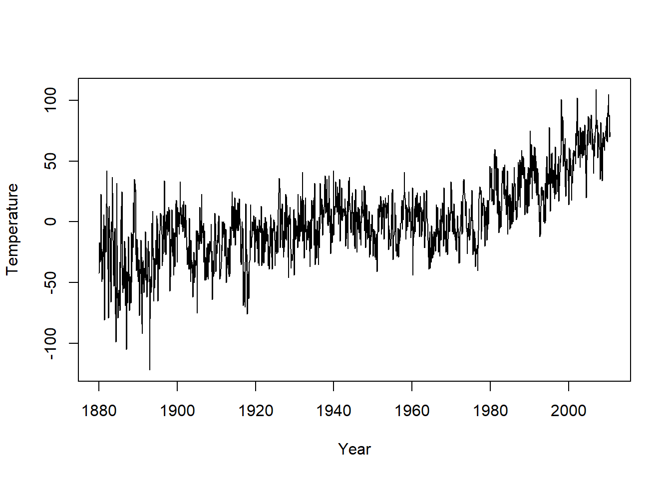
图16.1: 全球温度异常值月度时间序列
可以看到从1980年代开始有明显的上升趋势。 序列的波动性(方差)未见变大。
温度序列的ACF:
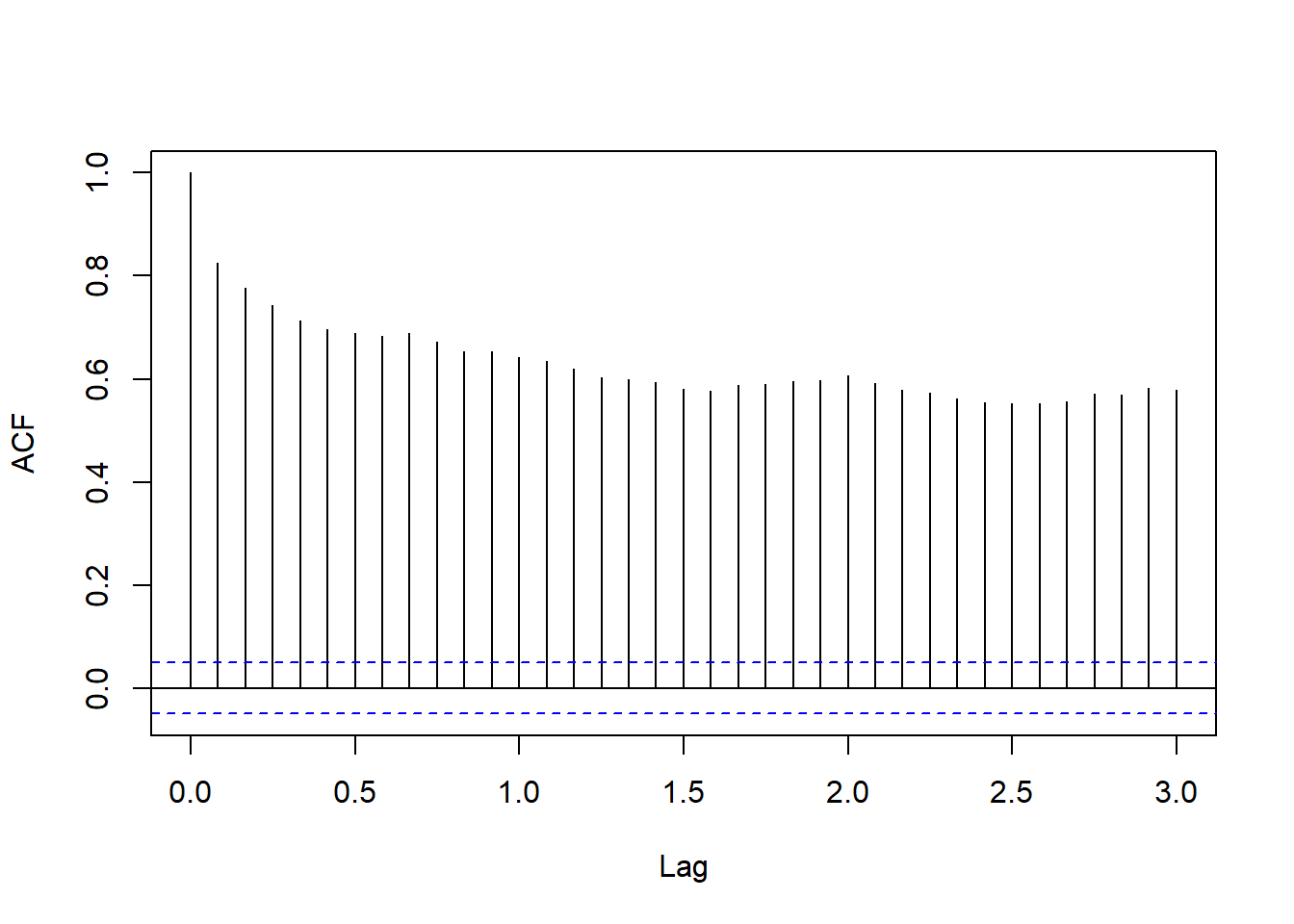
图16.2: 全球温度异常值的ACF
这样的ACF是缓慢下降的,一般为单位根非平稳或者有接近1的特征根的ARMA模型。
差分序列的时间序列图:
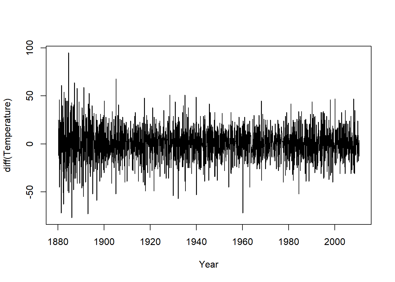
图16.3: 全球温度异常值的差分序列
差分序列的ACF:
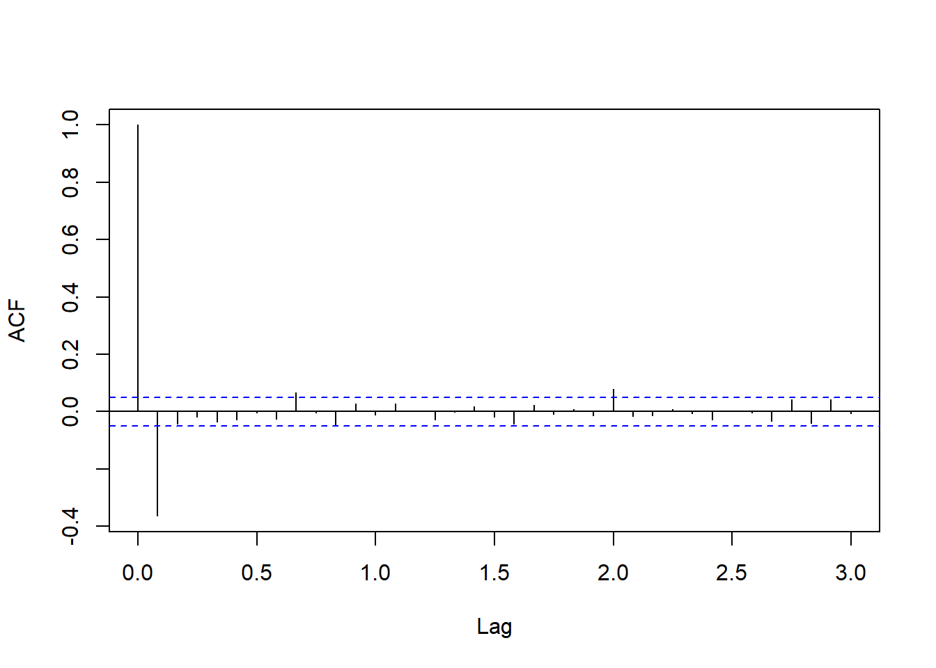
图16.4: 全球温度异常值差分序列的ACF
ACF是快速衰减的, 只有滞后1是明显显著的,其它滞后位置即使超过了0.05水平界限也仅是刚刚超过。 可以考虑MA(1)模型。
差分序列的PACF:

图16.5: 全球温度异常值差分序列的PACF
PACF是快速衰减的, 从PACF看不能用低阶AR建模。
16.2 单位根非平稳模型
做单位根检验:
##
## Call:
## ar(x = dG, method = "mle")
##
## Coefficients:
##       1        2        3        4        5        6        7        8
## -0.5435  -0.3826  -0.3091  -0.2942  -0.2819  -0.2409  -0.2035  -0.0986
##       9       10       11       12
## -0.0892  -0.1048  -0.0658  -0.0425
##
## Order selected 12 sigma^2 estimated as 275.1##
## Title:
## Augmented Dickey-Fuller Test
##
## Test Results:
## PARAMETER:
## Lag Order: 12
## STATISTIC:
## Dickey-Fuller: -2.7236
## P VALUE:
## 0.07438
##
## Description:
## Tue May 21 15:21:38 2024 by user: Lenovo## Warning in fUnitRoots::adfTest(Gtemp, lags = 12, type = "ct"): p-value smaller
## than printed p-value##
## Title:
## Augmented Dickey-Fuller Test
##
## Test Results:
## PARAMETER:
## Lag Order: 12
## STATISTIC:
## Dickey-Fuller: -5.5578
## P VALUE:
## 0.01
##
## Description:
## Tue May 21 15:21:38 2024 by user: Lenovo检验结果不确定是否有单位根。
因为序列有明显趋势, 而且ACF衰减缓慢, 考虑用单位根非平稳模型, 计算序列的差分。 记\(\{ G_t \}\)为温度异常值序列, 对\(\Delta G_t = G_t - G_{t-1}\)建模。
用AIC作AR定阶:
##
## Call:
## ar(x = dG, method = "mle")
##
## Coefficients:
##       1        2        3        4        5        6        7        8
## -0.5435  -0.3826  -0.3091  -0.2942  -0.2819  -0.2409  -0.2035  -0.0986
##       9       10       11       12
## -0.0892  -0.1048  -0.0658  -0.0425
##
## Order selected 12  sigma^2 estimated as  275.1
AIC给出12阶,因为是月度数据, 所以滞后12出现是合理的。 考察AR(12)的系数估计的SE:
##
## Call:
## arima(x = Gtemp, order = c(12, 1, 0))
##
## Coefficients:
##           ar1      ar2      ar3      ar4      ar5      ar6      ar7      ar8
##       -0.5359  -0.3774  -0.3081  -0.2924  -0.2773  -0.2366  -0.1995  -0.0969
## s.e.   0.0253   0.0286   0.0300   0.0309   0.0317   0.0321   0.0321   0.0317
##           ar9     ar10     ar11     ar12
##       -0.0913  -0.1153  -0.0644  -0.0422
## s.e.   0.0310   0.0301   0.0287   0.0253
##
## sigma^2 estimated as 275.2:  log likelihood = -6625.17,  aic = 13276.35
AR(12)的模型无法精简。 这个模型的阶数太高了。
考虑MA模型。MA(1):
##
## Call:
## arima(x = Gtemp, order = c(0, 1, 1))
##
## Coefficients:
##           ma1
##       -0.6038
## s.e.   0.0289
##
## sigma^2 estimated as 289.3:  log likelihood = -6664.07,  aic = 13332.14
MA(1)模型的AIC为13332.14, 不如AR(12)的13276.33。 考虑MA(2):
##
## Call:
## arima(x = Gtemp, order = c(0, 1, 2))
##
## Coefficients:
##           ma1      ma2
##       -0.5511  -0.1765
## s.e.   0.0241   0.0260
##
## sigma^2 estimated as 281.2:  log likelihood = -6641.88,  aic = 13289.76
MA(2)的AIC为13289.76, 还是不如AR(12)的13276.33。
考虑MA(12):
##
## Call:
## arima(x = Gtemp, order = c(0, 1, 12))
##
## Coefficients:
##           ma1      ma2      ma3      ma4      ma5      ma6     ma7     ma8
##       -0.5590  -0.1044  -0.0719  -0.0755  -0.0488  -0.0078  0.0027  0.0692
## s.e.   0.0254   0.0290   0.0292   0.0291   0.0291   0.0290  0.0302  0.0295
##           ma9     ma10    ma11     ma12
##       -0.0419  -0.0519  0.0191  -0.0474
## s.e.   0.0302   0.0279  0.0295   0.0268
##
## sigma^2 estimated as 269.7:  log likelihood = -6609.76,  aic = 13245.52
MA(12)的AIC为13245.52, 远好于AR(12)的13276.33。 拟合精简的MA(12):
##
## Call:
## arima(x = Gtemp, order = c(0, 1, 12), fixed = fixed)
##
## Coefficients:
##           ma1      ma2      ma3      ma4      ma5      ma6  ma7     ma8
##       -0.5589  -0.1043  -0.0718  -0.0754  -0.0486  -0.0070    0  0.0699
## s.e.   0.0254   0.0289   0.0292   0.0291   0.0290   0.0275    0  0.0285
##           ma9     ma10    ma11     ma12
##       -0.0417  -0.0517  0.0191  -0.0471
## s.e.   0.0302   0.0279  0.0295   0.0266
##
## sigma^2 estimated as 269.7: log likelihood = -6609.76, aic = 13243.53##
## Call:
## arima(x = Gtemp, order = c(0, 1, 12), fixed = fixed)
##
## Coefficients:
## ma1 ma2 ma3 ma4 ma5 ma6 ma7 ma8 ma9
## -0.5593 -0.1048 -0.0722 -0.076 -0.0516 0 0 0.0693 -0.0414
## s.e. 0.0254 0.0289 0.0294 0.029 0.0265 0 0 0.0285 0.0302
## ma10 ma11 ma12
## -0.0523 0.0182 -0.0473
## s.e. 0.0278 0.0293 0.0266
##
## sigma^2 estimated as 269.7: log likelihood = -6609.8, aic = 13241.59##
## Call:
## arima(x = Gtemp, order = c(0, 1, 12), fixed = fixed)
##
## Coefficients:
## ma1 ma2 ma3 ma4 ma5 ma6 ma7 ma8 ma9
## -0.5580 -0.1049 -0.0742 -0.0761 -0.0504 0 0 0.0699 -0.0385
## s.e. 0.0253 0.0290 0.0292 0.0290 0.0264 0 0 0.0286 0.0299
## ma10 ma11 ma12
## -0.0459 0 -0.0398
## s.e. 0.0258 0 0.0237
##
## sigma^2 estimated as 269.8: log likelihood = -6609.99, aic = 13239.98##
## Call:
## arima(x = Gtemp, order = c(0, 1, 12), fixed = fixed)
##
## Coefficients:
## ma1 ma2 ma3 ma4 ma5 ma6 ma7 ma8 ma9
## -0.5572 -0.1074 -0.0749 -0.0772 -0.0494 0 0 0.0544 0
## s.e. 0.0252 0.0289 0.0292 0.0287 0.0258 0 0 0.0258 0
## ma10 ma11 ma12
## -0.0615 0 -0.0440
## s.e. 0.0228 0 0.0235
##
## sigma^2 estimated as 270.1: log likelihood = -6610.82, aic = 13239.65最后选择了一个MA(12)限制滞后6、7、9、11系数为零。 考察这个模型的诊断:
fixed <- rep(NA_real_, 12)
fixed[c(6,7,11,9)] <- 0
mod1 <- arima(Gtemp, order=c(0,1,12), fixed=fixed)
forecast::checkresiduals(mod1, gof=36)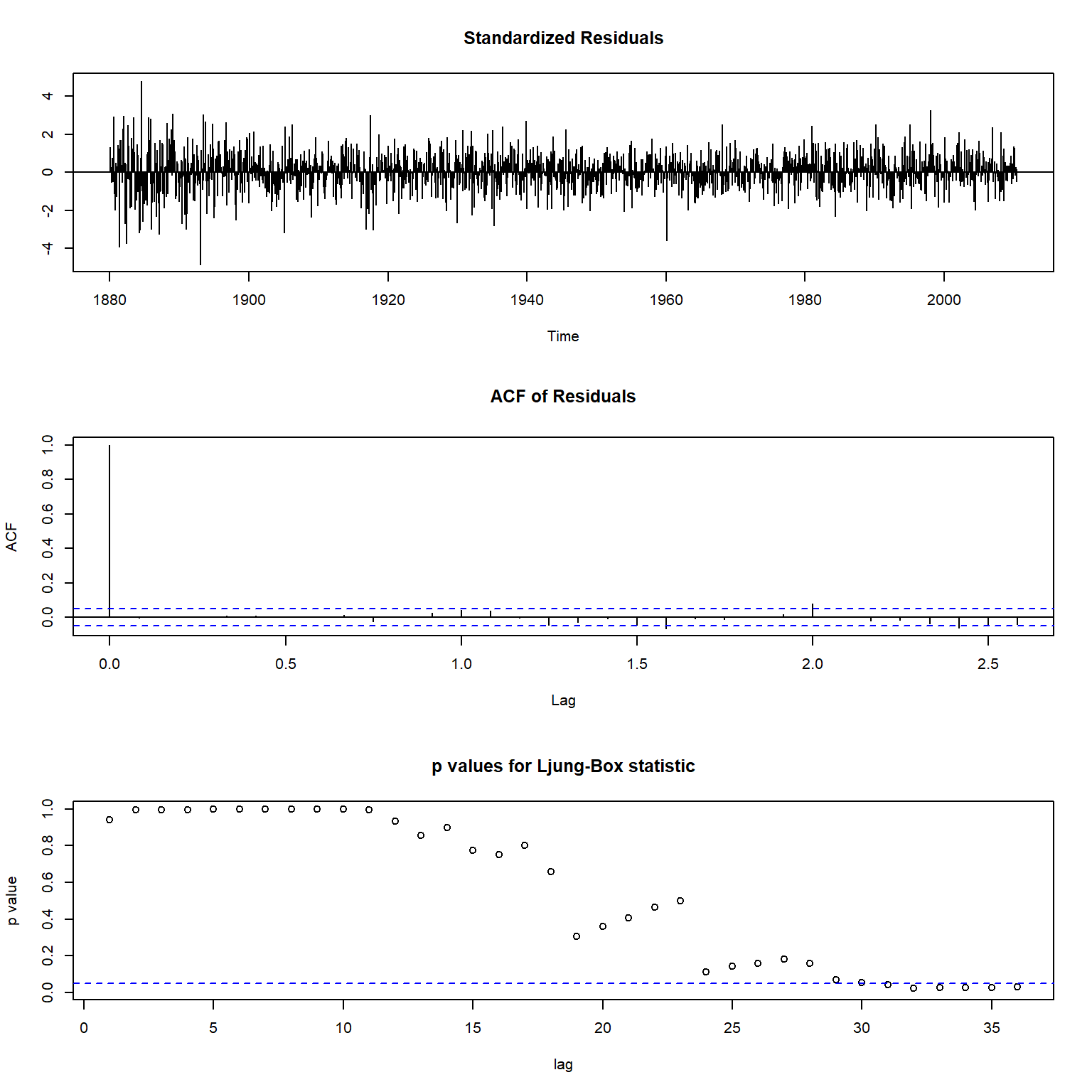
图16.6: 稀疏系数MA(12)模型诊断
##
##  Ljung-Box test
##
## data:  Residuals from ARIMA(0,1,12)
## Q* = 32.561, df = 12, p-value = 0.001133
##
## Model df: 12.   Total lags used: 24
残差有重尾现象,除此之外比较符合白噪声要求。 在Ljung-Box检验使用自相关系数个数很多时会有拒绝白噪声假设的问题。
考虑用ARMA。 ARIMA(1,1,1):
##
## Call:
## arima(x = Gtemp, order = c(1, 1, 1))
##
## Coefficients:
##          ar1      ma1
##       0.3759  -0.8879
## s.e.  0.0430   0.0281
##
## sigma^2 estimated as 277:  log likelihood = -6630.33,  aic = 13266.65
效果不如刚才的MA(12)。 考察其模型诊断:

##
##  Ljung-Box test
##
## data:  Residuals from ARIMA(1,1,1)
## Q* = 57.538, df = 22, p-value = 5.13e-05
##
## Model df: 2.   Total lags used: 24
模型诊断表明ARIMA(1,1,1)是不充分的。
考虑ARIMA(1,1,2)模型:
##
## Call:
## arima(x = Gtemp, order = c(1, 1, 2))
##
## Coefficients:
##          ar1      ma1     ma2
##       0.7387  -1.2973  0.3183
## s.e.  0.0406   0.0533  0.0492
##
## sigma^2 estimated as 272.1:  log likelihood = -6616.56,  aic = 13241.11
其AIC为13241.11, 比稀疏系数MA(12)的13239.65略差, 但是模型更简单。 作模型诊断:

##
##  Ljung-Box test
##
## data:  Residuals from ARIMA(1,1,2)
## Q* = 39.558, df = 21, p-value = 0.008413
##
## Model df: 3.   Total lags used: 24
Ljung-Box检验的结果比MA(12)的结果差。
尝试加入一个季节MA项:
##
## Call:
## arima(x = Gtemp, order = c(1, 1, 2), seasonal = list(order = c(0, 0, 1), period = 12))
##
## Coefficients:
##          ar1      ma1     ma2    sma1
##       0.7409  -1.3002  0.3206  0.0128
## s.e.  0.0400   0.0529  0.0490  0.0239
##
## sigma^2 estimated as 272:  log likelihood = -6616.41,  aic = 13242.81
加入的季节MA系数不显著,AIC变差一些。 继续尝试加入滞后24的季节MA:
##
## Call:
## arima(x = Gtemp, order = c(1, 1, 2), seasonal = list(order = c(0, 0, 2), period = 12))
##
## Coefficients:
##          ar1      ma1     ma2    sma1    sma2
##       0.7619  -1.3256  0.3426  0.0147  0.0717
## s.e.  0.0374   0.0514  0.0482  0.0257  0.0243
##
## sigma^2 estimated as 270.5:  log likelihood = -6612.04,  aic = 13236.07
mod2 <- arima(Gtemp, order=c(1,1,2),
seasonal=list(order=c(0,0,2), period=12),
fixed=c(NA, NA, NA, 0, NA))
mod2##
## Call:
## arima(x = Gtemp, order = c(1, 1, 2), seasonal = list(order = c(0, 0, 2), period = 12),
## fixed = c(NA, NA, NA, 0, NA))
##
## Coefficients:
## ar1 ma1 ma2 sma1 sma2
## 0.7612 -1.3241 0.3416 0 0.0717
## s.e. 0.0379 0.0519 0.0485 0 0.0243
##
## sigma^2 estimated as 270.6: log likelihood = -6612.2, aic = 13234.4此模型的AIC在比较的模型中最优。 进行模型诊断:
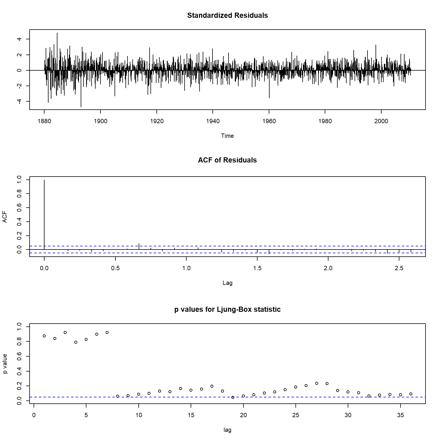
图16.7: ARIMA\((1,1,2)(0,0,2)_{12}\)模型诊断
##
##  Ljung-Box test
##
## data:  Residuals from ARIMA(1,1,2)(0,0,2)[12]
## Q* = 31.102, df = 19, p-value = 0.03934
##
## Model df: 5.   Total lags used: 24
模型诊断图表明模型基本充分, 但也有一些缺陷:残差可能存在较多异常值, LB白噪声检验结果接近于拒绝白噪声假设。 在单位根非平稳模型中可以选定这个模型。 模型写成:
\[ (1 - 0.7612 B)(1-B) G_t = (1 + 0.0717 B^{24})(1 - 1.3241 B + 0.3416 B^2) \varepsilon_t, \\ \ \text{Var}(\varepsilon_t) = 270.6 \]
AIC值为11234.4。
16.3 线性固定趋势模型
由于温度时间序列存在明显的上升趋势, 一种候选模型是固定趋势模型。 最简单的固定趋势是线性趋势:
\[ G_t = \beta_0 + \beta_1 t + z_t \]
其中\(\{ z_t \}\)为线性时间序列。
先做简单的回归:
##
## Call:
## lm(formula = c(Gtemp) ~ tt)
##
## Residuals:
##     Min      1Q  Median      3Q     Max
## -92.055 -15.634   0.194  15.296  78.751
##
## Coefficients:
##               Estimate Std. Error t value Pr(>|t|)
## (Intercept) -38.039763   1.134960  -33.52   <2e-16 ***
## tt            0.051560   0.001253   41.15   <2e-16 ***
## ---
## Signif. codes:  0 '***' 0.001 '**' 0.01 '*' 0.05 '.' 0.1 ' ' 1
##
## Residual standard error: 22.46 on 1566 degrees of freedom
## Multiple R-squared:  0.5195, Adjusted R-squared:  0.5192
## F-statistic:  1693 on 1 and 1566 DF,  p-value: < 2.2e-16
将估计的趋势叠加到原始序列图形上面:
plot(tt, Gtemp, type="l", xlab="Time", ylab="Temperature", main="Fixed Linear Trend")
abline(reslm, lwd=2, col="red")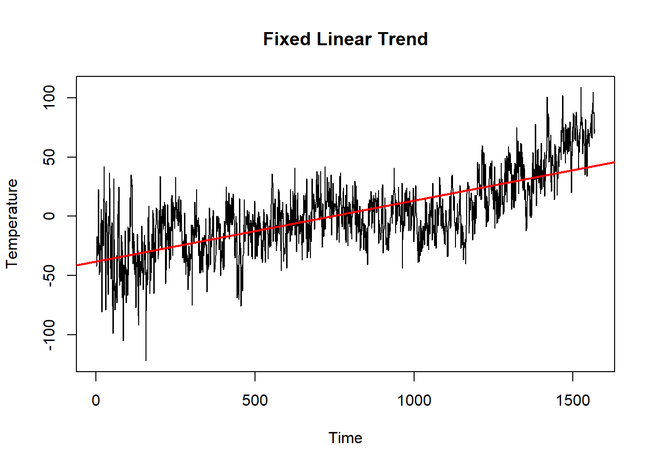
图16.8: 非随机线性趋势
这个模型拟合的效果还是不够精细。 后面可以再设法改进。
考察回归的残差。 残差序列图:
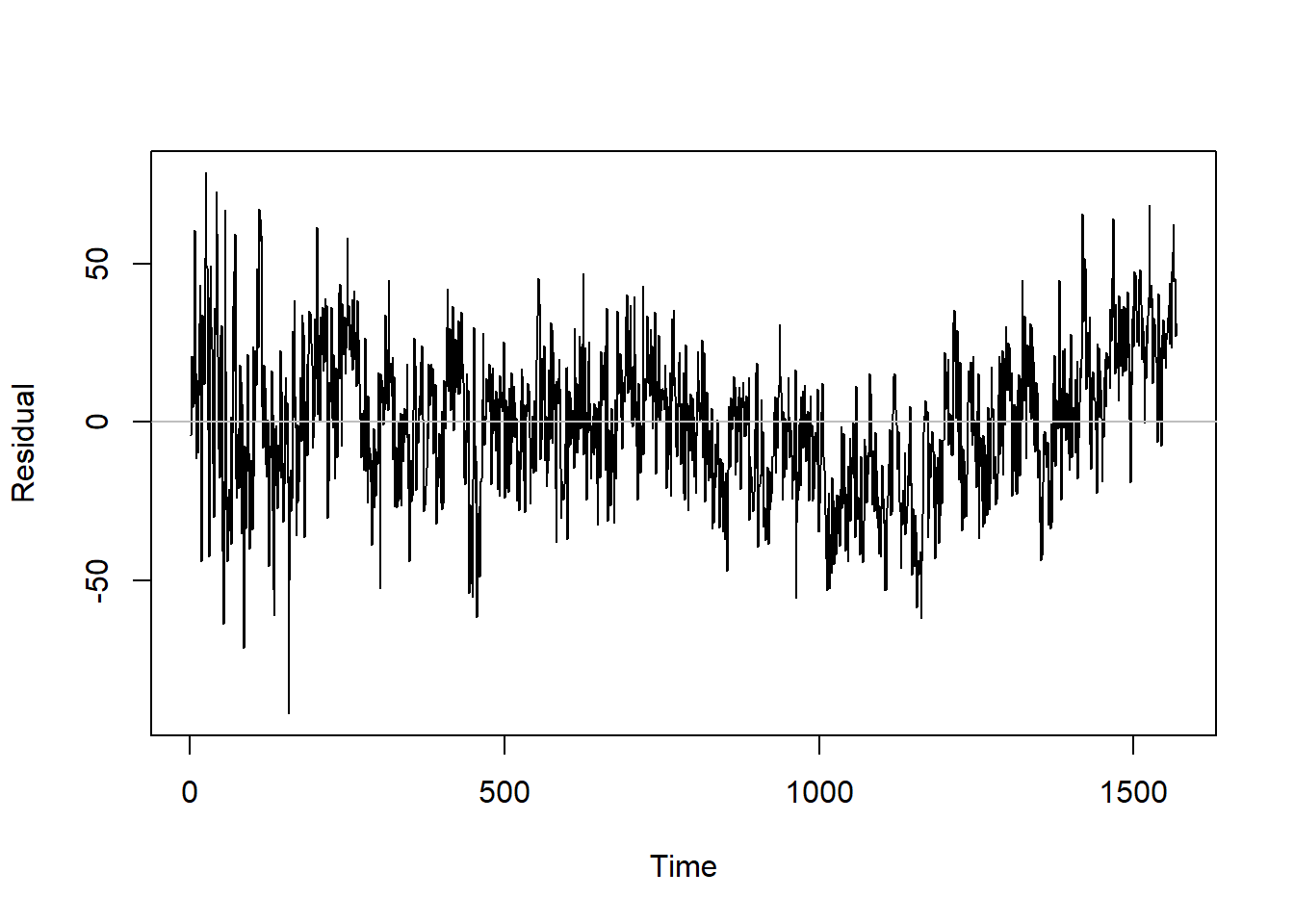
图16.9: 非随机线性趋势残差序列
残差序列的ACF:
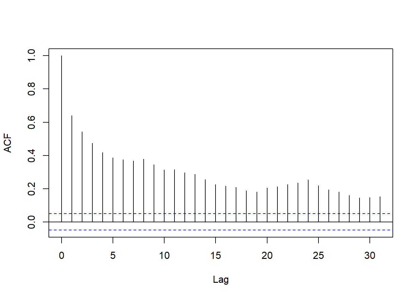
图16.10: 非随机线性趋势残差序列ACF
基本可以算是快速衰减,但不能用低阶MA表示。
残差序列的PACF:
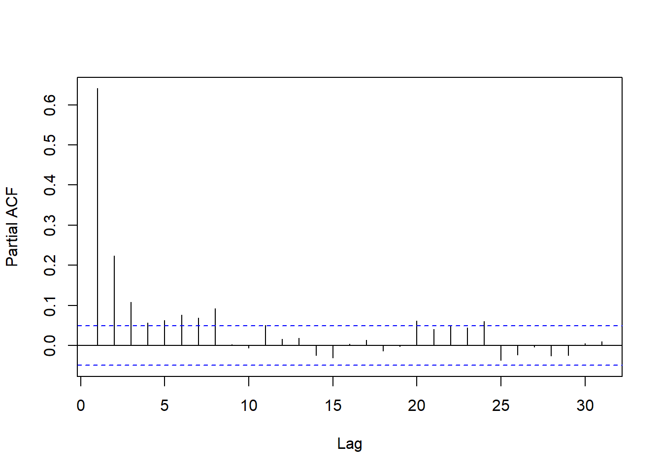
图16.11: 非随机线性趋势残差序列PACF
可以算是快速衰减, 用低阶AR建模也有一定困难。
从回归残差看可以认为残差是线性平稳列, 称这样的\(G_t\)为趋势平稳序列。
对回归残差采用ARMA(2,1)模型:
##
## Call:
## arima(x = Gtemp, order = c(2, 0, 1), xreg = tt)
##
## Coefficients:
##          ar1      ar2      ma1  intercept      tt
##       1.2385  -0.2719  -0.7802   -38.8493  0.0530
## s.e.  0.0567   0.0477   0.0460     5.3548  0.0059
##
## sigma^2 estimated as 272.9:  log likelihood = -6622.99,  aic = 13257.97
模型可以写成
\[ \begin{aligned} G_t =& -38.8493 + 0.0530 t + z_t \\ z_t =& 1.2385 z_{t-1} - 0.2719 z_{t-2} + \varepsilon_t - 0.7802 \varepsilon_{t-1}, \ \text{Var}(\varepsilon_t) = 272.9 \end{aligned} \]
对其进行模型诊断:
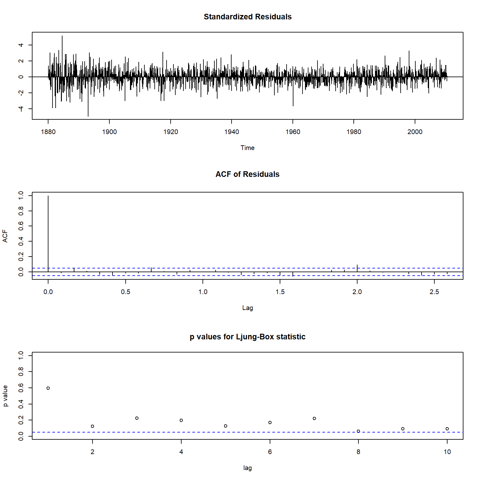
图16.12: 线性趋势模型诊断
##
##  Ljung-Box test
##
## data:  Residuals from ARIMA(2,0,1) with non-zero mean
## Q* = 46.125, df = 21, p-value = 0.00123
##
## Model df: 3.   Total lags used: 24
结果基本可以接受, ACF在滞后24处略超出0.05界限。 考虑加入滞后24的MA项看是否有改进:
tt <- seq(length(Gtemp))
resm <- arima(Gtemp, xreg=tt, order=c(2,0,1),
              seasonal=list(order=c(0,0,2), period=12)); resm
##
## Call:
## arima(x = Gtemp, order = c(2, 0, 1), seasonal = list(order = c(0, 0, 2), period = 12),
## xreg = tt)
##
## Coefficients:
## ar1 ar2 ma1 sma1 sma2 intercept tt
## 1.1935 -0.2376 -0.7426 0.0043 0.0856 -38.6296 0.0528
## s.e. 0.0607 0.0494 0.0505 0.0265 0.0241 5.1662 0.0057
##
## sigma^2 estimated as 270.7: log likelihood = -6616.71, aic = 13249.42mod4 <- arima(Gtemp, xreg=tt, order=c(2,0,1), fixed=c(NA, NA, NA, 0, NA, NA, NA),
seasonal=list(order=c(0,0,2), period=12)); mod4##
## Call:
## arima(x = Gtemp, order = c(2, 0, 1), seasonal = list(order = c(0, 0, 2), period = 12),
## xreg = tt, fixed = c(NA, NA, NA, 0, NA, NA, NA))
##
## Coefficients:
## ar1 ar2 ma1 sma1 sma2 intercept tt
## 1.1960 -0.2394 -0.7451 0 0.0856 -38.7150 0.0529
## s.e. 0.0587 0.0482 0.0486 0 0.0241 5.1843 0.0057
##
## sigma^2 estimated as 270.8: log likelihood = -6616.72, aic = 13247.45从AIC来看是有明显改进的。 但是,AIC比较不如单位根非平稳模型的结果。 模型为:
\[ \begin{aligned} G_t =& -38.7150 + 0.0529 t + z_t \\ (1 -1.1960B + 0.2394B^2)z_t =& (1 - 0.7451B)(1 + 0.0856B^{24})\varepsilon_t, \ \text{Var}(\varepsilon_t) = 270.8 \end{aligned} \]
对此模型的残差诊断图:

图16.13: 趋势平稳改进模型的诊断图
##
##  Ljung-Box test
##
## data:  Residuals from ARIMA(2,0,1)(0,0,2)[12] with non-zero mean
## Q* = 30.064, df = 19, p-value = 0.05099
##
## Model df: 5.   Total lags used: 24
结果表明模型比较充分。 在趋势平稳假定下选择这个模型。
从估计结果看, 平均每月气温增长0.000529摄氏度, 平均每年气温增长0.006348摄氏度, 平均158年增加1摄氏度。
16.4 二次固定趋势模型
温度异常值时间序列的增长趋势不像是线性的, 在最后四十年增长更快。 比较简单的非线性函数是二次多项式函数。 模型为 \[ G_t = \beta_0 + \beta_1 t + \beta_2 t^2 + z_t \]
其中\(\{ z_t \}\)为线性时间序列。
先做简单的回归:
##
## Call:
## lm(formula = c(Gtemp) ~ tt + I(tt^2))
##
## Residuals:
##    Min     1Q Median     3Q    Max
## -99.53 -14.45   1.10  14.68  64.02
##
## Coefficients:
##               Estimate Std. Error t value Pr(>|t|)
## (Intercept) -2.178e+01  1.613e+00 -13.505   <2e-16 ***
## tt          -1.058e-02  4.748e-03  -2.228    0.026 *
## I(tt^2)      3.960e-05  2.930e-06  13.517   <2e-16 ***
## ---
## Signif. codes:  0 '***' 0.001 '**' 0.01 '*' 0.05 '.' 0.1 ' ' 1
##
## Residual standard error: 21.26 on 1565 degrees of freedom
## Multiple R-squared:  0.5697, Adjusted R-squared:  0.5692
## F-statistic:  1036 on 2 and 1565 DF,  p-value: < 2.2e-16
将估计的趋势叠加到原始序列图形上面:
plot(tt, Gtemp, type="l", xlab="Time", ylab="Temperature", main="Fixed Quadratic Trend")
lines(tt, predict(reslm2), lwd=2, col="blue")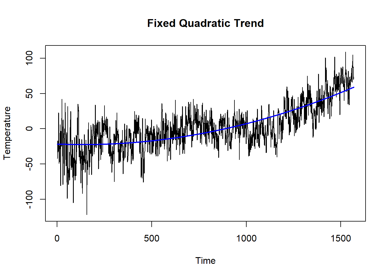
图16.14: 非随机二次多项式趋势
考察回归的残差。 残差序列图:
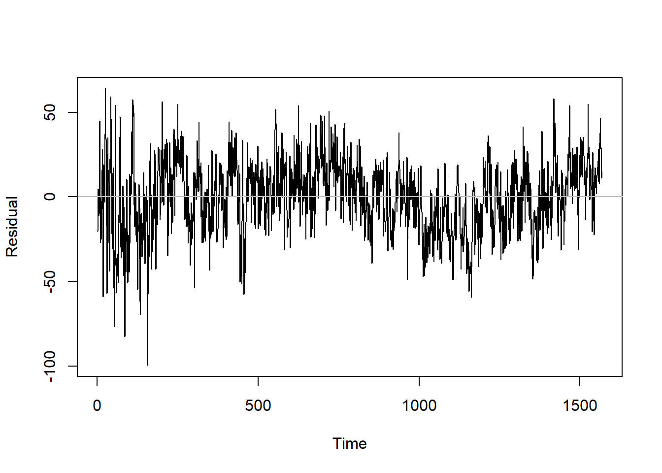
图16.15: 非随机二次多项式趋势残差序列
残差序列仍呈现出非平稳。
残差序列的ACF:
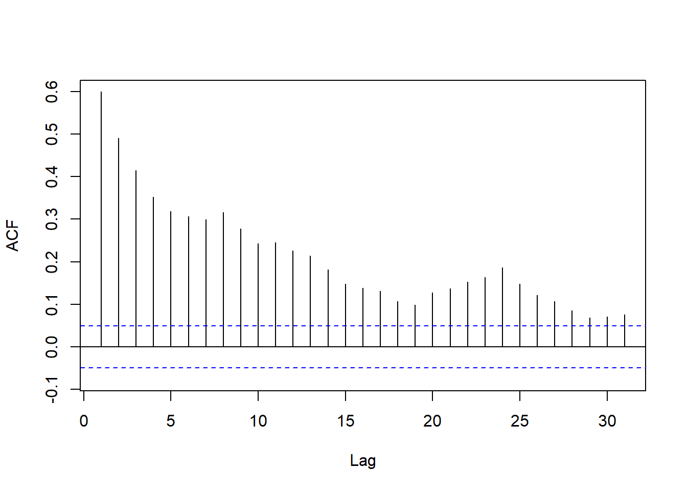
图16.16: 非随机线性趋势残差序列ACF
此ACF不能用低阶MA表示。 PACF为:

图16.17: 非随机线性趋势残差序列PACF
PACF表现像是低阶AR模型。
用AIC确定一个AR模型:
##
## Call:
## ar(x = reslm2$residuals, method = "mle")
##
## Coefficients:
##      1       2       3       4       5       6       7       8
## 0.4363  0.1413  0.0593  0.0071  0.0074  0.0286  0.0238  0.0901
##
## Order selected 8 sigma^2 estimated as 268.5用arima()函数联合估计:
tt <- seq(length(Gtemp))
tt2 <- (tt - mean(tt))^2/1E5
mod5 <- arima(Gtemp, xreg=cbind(tt, tt2), order=c(8,0,0)); mod5
##
## Call:
## arima(x = Gtemp, order = c(8, 0, 0), xreg = cbind(tt, tt2))
##
## Coefficients:
## ar1 ar2 ar3 ar4 ar5 ar6 ar7 ar8 intercept
## 0.4361 0.1415 0.0594 0.0070 0.0075 0.0286 0.0240 0.0896 -46.8156
## s.e. 0.0251 0.0275 0.0277 0.0277 0.0277 0.0277 0.0275 0.0252 4.5405
## tt tt2
## 0.0522 4.0754
## s.e. 0.0044 1.0620
##
## sigma^2 estimated as 268.5: log likelihood = -6610.02, aic = 13244.03对残差考虑ARMA建模。 ARMA(1,1):
tt <- seq(length(Gtemp))
tt2 <- (tt - mean(tt))^2/1E5
resm <- arima(Gtemp, xreg=cbind(tt, tt2), order=c(1,0,1)); resm
##
## Call:
## arima(x = Gtemp, order = c(1, 0, 1), xreg = cbind(tt, tt2))
##
## Coefficients:
## ar1 ma1 intercept tt tt2
## 0.8476 -0.4199 -46.4231 0.0519 3.9788
## s.e. 0.0223 0.0410 3.6182 0.0035 0.8538
##
## sigma^2 estimated as 273.3: log likelihood = -6623.93, aic = 13259.85效果不如AR(8)。 改为ARMA(1,2):
tt <- seq(length(Gtemp))
tt2 <- (tt - mean(tt))^2/1E5
resm <- arima(Gtemp, xreg=cbind(tt, tt2), order=c(1,0,2)); resm
##
## Call:
## arima(x = Gtemp, order = c(1, 0, 2), xreg = cbind(tt, tt2))
##
## Coefficients:
## ar1 ma1 ma2 intercept tt tt2
## 0.9003 -0.4637 -0.0954 -46.6156 0.0521 4.0167
## s.e. 0.0227 0.0363 0.0332 4.1794 0.0040 0.9814
##
## sigma^2 estimated as 272: log likelihood = -6620.18, aic = 13254.37改为ARMA(2,1):
tt <- seq(length(Gtemp))
tt2 <- (tt - mean(tt))^2/1E5
resm <- arima(Gtemp, xreg=cbind(tt, tt2), order=c(2,0,1)); resm
##
## Call:
## arima(x = Gtemp, order = c(2, 0, 1), xreg = cbind(tt, tt2))
##
## Coefficients:
## ar1 ar2 ma1 intercept tt tt2
## 1.1946 -0.2460 -0.7454 -46.8246 0.0522 4.0737
## s.e. 0.0651 0.0513 0.0554 4.6574 0.0045 1.0875
##
## sigma^2 estimated as 271.1: log likelihood = -6617.5, aic = 13249增加一个滞后24的季节MA项:
tt <- seq(length(Gtemp))
tt2 <- (tt - mean(tt))^2/1E5
resm <- arima(Gtemp, xreg=cbind(tt, tt2), order=c(2,0,1),
              seasonal=list(order=c(0,0,2), period=12))
resm
##
## Call:
## arima(x = Gtemp, order = c(2, 0, 1), seasonal = list(order = c(0, 0, 2), period = 12),
## xreg = cbind(tt, tt2))
##
## Coefficients:
## ar1 ar2 ma1 sma1 sma2 intercept tt tt2
## 1.1527 -0.2156 -0.7104 0.0078 0.0848 -46.8806 0.0523 4.1021
## s.e. 0.0691 0.0529 0.0599 0.0265 0.0239 4.7049 0.0045 1.0983
##
## sigma^2 estimated as 268.9: log likelihood = -6611.15, aic = 13240.31删去SMA1系数:
tt <- seq(length(Gtemp))
tt2 <- (tt - mean(tt))^2/1E5
fixed <- rep(NA_real_, 8)
fixed[4] <- 0
mod6 <- arima(Gtemp, xreg=cbind(tt, tt2), order=c(2,0,1),
              seasonal=list(order=c(0,0,2), period=12),
              fixed=fixed)
mod6
##
## Call:
## arima(x = Gtemp, order = c(2, 0, 1), seasonal = list(order = c(0, 0, 2), period = 12),
## xreg = cbind(tt, tt2), fixed = fixed)
##
## Coefficients:
## ar1 ar2 ma1 sma1 sma2 intercept tt tt2
## 1.1568 -0.2183 -0.7141 0 0.0849 -46.8836 0.0522 4.1094
## s.e. 0.0666 0.0515 0.0574 0 0.0239 4.7189 0.0045 1.1014
##
## sigma^2 estimated as 268.9: log likelihood = -6611.2, aic = 13238.4方程可以写成:
\[ G_t = -46.88 + 0.0522 t + 4.109\times 10^{-5} (t - 784.5)^2 + z_t \\ z_t = 1.16 z_{t-1} - 0.22 z_{t-2} + (1 - 0.7141B)(1 + 0.0849B^{24}) \varepsilon_t \\ \text{Var}(\varepsilon_t)=268.9 \]
模型的残差诊断:
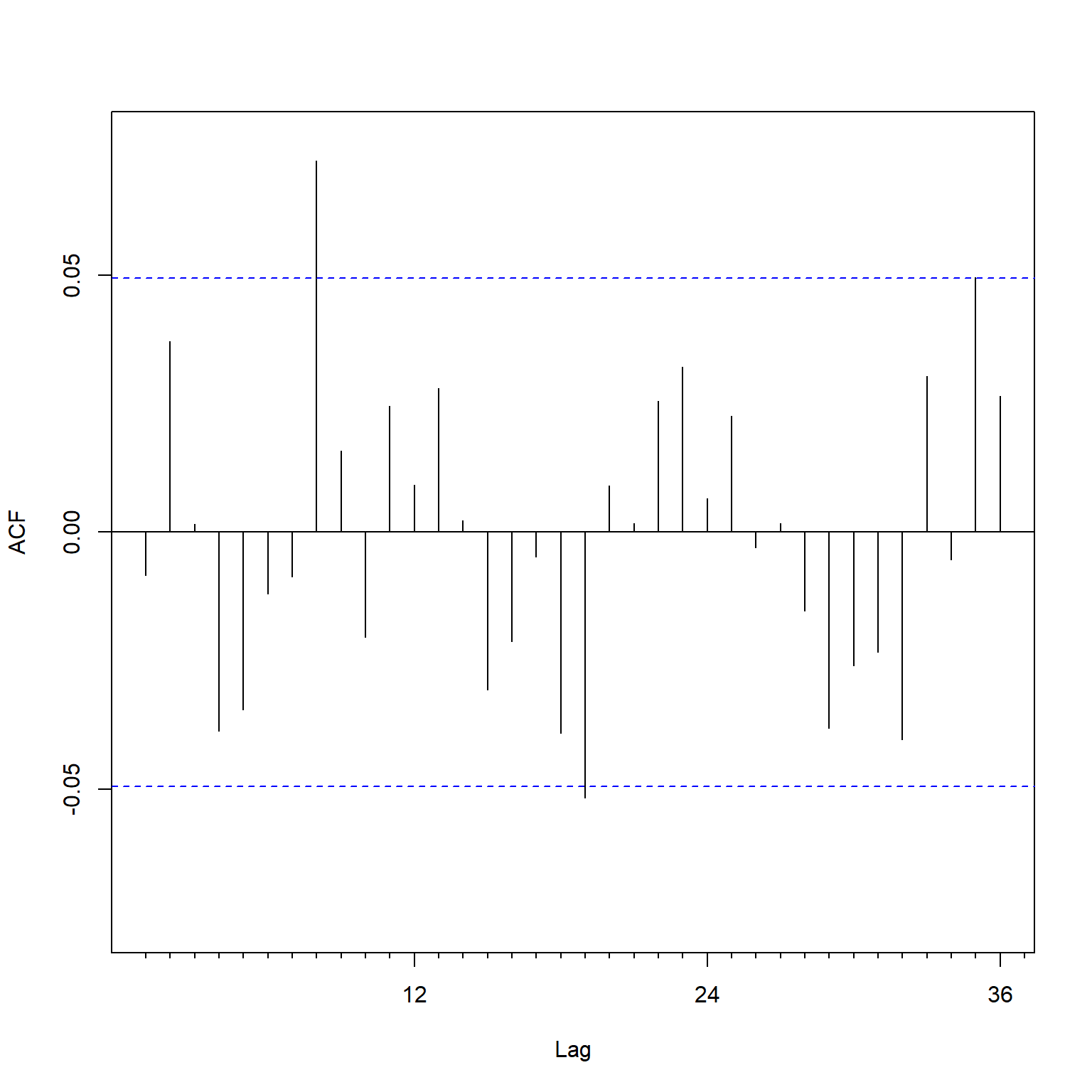
图16.18: 二次趋势模型建模的残差诊断
16.5 模型比较
前面考虑了多个模型,以下的三个模型是选择出来较好的, 对模型残差的检验也能证明模型充分。 如何比较效果相近的模型?
使用差分平稳模型(随机趋势模型)时, 选用ARIMA\((1,1,2)(0,0,2)_{12}\)且季节MA滞后1系数为零。
mc1 <- arima(
  Gtemp, order=c(1,1,2),
  seasonal=list(order=c(0,0,2), period=12),
  fixed=c(NA, NA, NA, 0, NA))
mc1
##
## Call:
## arima(x = Gtemp, order = c(1, 1, 2), seasonal = list(order = c(0, 0, 2), period = 12),
## fixed = c(NA, NA, NA, 0, NA))
##
## Coefficients:
## ar1 ma1 ma2 sma1 sma2
## 0.7612 -1.3241 0.3416 0 0.0717
## s.e. 0.0379 0.0519 0.0485 0 0.0243
##
## sigma^2 estimated as 270.6: log likelihood = -6612.2, aic = 13234.4使用非随机线性趋势模型时, 残差选用ARIMA\((2,0,1)(0,0,2)_{12}\)且季节MA滞后1系数为零。
tt <- seq(length(Gtemp))
mc2 <- arima(
  Gtemp,
  xreg=tt,
  order=c(2,0,1),
  seasonal=list(order=c(0,0,2), period=12),
  fixed=c(NA, NA, NA, 0, NA, NA, NA))
mc2
##
## Call:
## arima(x = Gtemp, order = c(2, 0, 1), seasonal = list(order = c(0, 0, 2), period = 12),
## xreg = tt, fixed = c(NA, NA, NA, 0, NA, NA, NA))
##
## Coefficients:
## ar1 ar2 ma1 sma1 sma2 intercept tt
## 1.1960 -0.2394 -0.7451 0 0.0856 -38.7150 0.0529
## s.e. 0.0587 0.0482 0.0486 0 0.0241 5.1843 0.0057
##
## sigma^2 estimated as 270.8: log likelihood = -6616.72, aic = 13247.45使用非随机二次多项式趋势模型时, 残差选用ARIMA\((2,0,1)(0,0,2)_{12}\)且季节MA滞后1系数为零。
tt <- seq(length(Gtemp))
tt2 <- (tt - mean(tt))^2/1E5
fixed <- rep(NA_real_, 8)
fixed[4] <- 0
mc3 <- arima(
  Gtemp, xreg=cbind(tt, tt2), order=c(2,0,1),
  seasonal=list(order=c(0,0,2), period=12),
  fixed=fixed)
mc3
##
## Call:
## arima(x = Gtemp, order = c(2, 0, 1), seasonal = list(order = c(0, 0, 2), period = 12),
## xreg = cbind(tt, tt2), fixed = fixed)
##
## Coefficients:
## ar1 ar2 ma1 sma1 sma2 intercept tt tt2
## 1.1568 -0.2183 -0.7141 0 0.0849 -46.8836 0.0522 4.1094
## s.e. 0.0666 0.0515 0.0574 0 0.0239 4.7189 0.0045 1.1014
##
## sigma^2 estimated as 268.9: log likelihood = -6611.2, aic = 13238.416.5.1 样本内比较
可以用对建模用数据的拟合情况比较模型优劣, 在所用的参数个数相近的情况下比较是有意义的。
比较可以用:
- 模型残差更符合白噪声特征;
- AIC或BIC更小;
- \(\sigma_{\varepsilon_t}^2\)更小。
从AIC来看, 应该是MC1的随机趋势模型最好, 其AIC=13234最小。
但是,不同的模型有完全不同的含义。 对于随机趋势模型, 它可以拟合出增长趋势, 但是模型并不意味着以后也会持续增长, 差分平稳模型完全可以表现出下降趋势。
对于非随机线性增长趋势模型, 因为有一个显著的线性增长项, 模型意味着以后温度也持续线性增长, 增长速度为每年0.00635度, 平均157年增长1摄氏度。
对于非随机二次增长趋势模型, 因为有一个显著的二次增长项, 模型意味着以后温度会加速增长, 从数据末尾的2010年8月的异常值74开始, 增加1摄氏度只需87年。
从现有的数据无法确定随机趋势模型还是非随机趋势模型更正确, 相对于全球温度变化这种缓慢变化, 现有的130数据还是太少了, 不足以反映整个历史中或较近的历史中的全球气温变化。 就好比我们在三年的时间观测到了股市为牛市, 就断言后面也是牛市一样不可信。
16.5.2 样本外比较
样本外比较的思想是, 建模时留出最后一部分时间不用于建模, 建模后对留出的时间做超前一步预报, 比较平均预报误差。
共有1568个月的数据, 取最后的200个月的数据作为验证。
使用MC1作预测的函数:
pred1 <- function(y=Gtemp, n.pred=200, DEBUG=FALSE){
  T <- length(y)
  ypred <- rep(NA_real_, T)
  step <- 0
  for(h in (T-n.pred):(T-1)){
    step <- step + 1
    if(DEBUG){
      cat("pred1: step", step, "/", n.pred, "\n")
    }
    mod <- arima(y[1:h], order=c(1,1,2),
             seasonal=list(order=c(0,0,2), period=12),
             fixed=c(NA, NA, NA, 0, NA))
    ypred[h+1] <- predict(mod, n.ahead=1, se.fit=FALSE)
  }

  ypred
}
使用MC2作预测的函数:
pred2 <- function(y=Gtemp, n.pred=200, DEBUG=FALSE){
  T <- length(y)
  ypred <- rep(NA_real_, T)
  step <- 0
  for(h in (T-n.pred):(T-1)){
    step <- step + 1
    if(DEBUG){
      cat("pred2: step", step, "/", n.pred, "\n")
    }
    tt <- seq(h)
    mod <- arima(y[1:h],
                 xreg=tt,
                 order=c(2,0,1),
                 seasonal=list(order=c(0,0,2), period=12),
                 fixed=c(NA, NA, NA, 0, NA, NA, NA))
    ypred[h+1] <- predict(mod, n.ahead=1, se.fit=FALSE,
                          newxreg=c(h+1))
  }

  ypred
}
使用MC3作预测的函数:
pred3 <- function(y=Gtemp, n.pred=200, DEBUG=FALSE){
  T <- length(y)
  ypred <- rep(NA_real_, T)
  fixed <- rep(NA_real_, 8)
  fixed[4] <- 0
  step <- 0
  for(h in (T-n.pred):(T-1)){
    step <- step + 1
    if(DEBUG){
      cat("pred3: step", step, "/", n.pred, "\n")
    }
    tt <- seq(h)
    tt2 <- (tt - 784.5)^2 * 1E-5

    mod <- arima(y[1:h],
                 xreg=cbind(tt, tt2),
                 order=c(2,0,1),
                 seasonal=list(order=c(0,0,2), period=12),
                 fixed=fixed)
    ypred[h+1] <- predict(
      mod, n.ahead=1, se.fit=FALSE,
      newxreg=cbind(tt=h+1, tt2=(h+1-784.5)^2 * 1E-5))
  }

  ypred
}
对一种方法的预测计算预测根均方误差(RMFSE)和平均绝对预测误差(MAFE)的函数:
pred.err <- function(y=Gtemp, n.pred=200, ypred){
  T <- length(y)
  i1 <- T - n.pred + 1
  RMFSE <- sqrt( mean((y[i1:T] - ypred[i1:T])^2) )
  MAFE <- mean(abs(y[i1:T] - ypred[i1:T]))

  c(RMFSE=RMFSE, MAFE=MAFE)
}
计算这三个候选模型的预测误差指标:
time_start <- proc.time()[3]
pred.tab <- data.frame(
  "模型"=paste("MC", 1:3, sep=""),
  RMFSE=rep(0.0, 3),
  MAFE=rep(0.0, 3)
)
funcs <- list(pred1, pred2, pred3)
for(i in 1:3){
  predf <- funcs[[i]]
  ypred <- predf(y=Gtemp, n.pred=200, DEBUG=TRUE)
  err <- pred.err(y=Gtemp, n.pred=200, ypred=ypred)
  pred.tab[i, "RMFSE"] <- err["RMFSE"]
  pred.tab[i, "MAFE"] <- err["MAFE"]
}
time_used <- proc.time()[3] - time_start
cat("回测检验花费时间:", round(time_used/60), "分钟\n")
## 回测检验花费时间: 10 分钟
预测误差比较的结果表格:
| 模型 | RMFSE | MAFE |
|---|---|---|
| MC1 | 14.53 | 11.17 |
| MC2 | 15.34 | 11.97 |
| MC3 | 14.87 | 11.51 |
样本外预测的结果也是随机趋势模型MC1最好。
16.6 长期预测
用MC1作超前1到1200步(共100年)的长期预测, 并作图:
pred.long1 <- function(y=Gtemp, n.pred=1200){
  T <- length(y)
  ypred <- ts(c(y, rep(NA_real_, n.pred)),
              start=start(y), frequency = frequency(y))
  ntotal <- T + n.pred
  lb <- ts(rep(NA_real_, ntotal),
           start=start(y), frequency = frequency(y))
  ub <- lb
  mod <- arima(
    y, order=c(1,1,2),
    seasonal=list(order=c(0,0,2), period=12),
    fixed=c(NA, NA, NA, 0, NA))
  ypred0 <- predict(mod, n.ahead=n.pred, se.fit=TRUE)
  ypred[(T+1):(T+n.pred)] <- ypred0$pred
  lb[(T+1):(T+n.pred)] <- ypred0$pred - 2*ypred0$se
  ub[(T+1):(T+n.pred)] <- ypred0$pred + 2*ypred0$se

  list(pred=ypred, lb=lb, ub=ub)
}
plot.pred <- function(y=Gtemp, pred.long=pred.long1, n.pred=1200){
ypred <- pred.long(y=Gtemp, n.pred=1200)
ylim <- range(c(ypred$pred, ypred$lb, ypred$ub), na.rm=TRUE)
times <- c(time(ypred$pred))
plot(times, ypred$pred, type="l", xlab="year", ylab="Forcast",
ylim=ylim)
t1 <- length(y)+1
t2 <- length(ypred$pred)
lines(times[t1:t2], ypred$pred[t1:t2], col="red")
lines(times[t1:t2], ypred$lb[t1:t2], lty=2, col="blue")
lines(times[t1:t2], ypred$ub[t1:t2], lty=2, col="blue")
}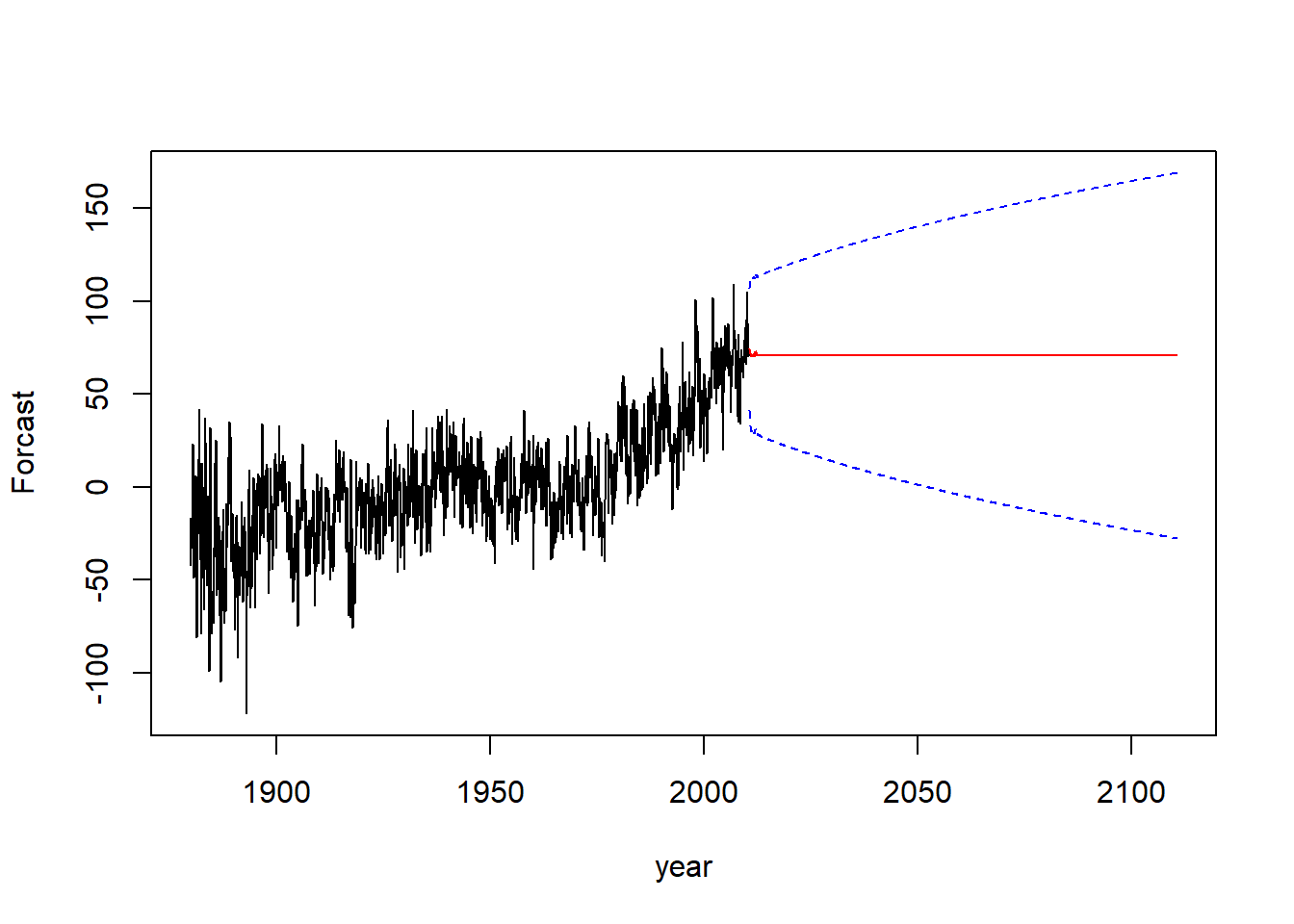
图16.19: 随机趋势模型的100年长期预测
可见随机趋势的预测结果基本是用最后一个有数据的月份的数据作为预测值, 预测的区间越来越宽。
用MC3作超前1到1200步(共100年)的长期预测, 并作图:
pred.long3 <- function(y=Gtemp, n.pred=1200){
  T <- length(y)
  ypred <- ts(c(y, rep(NA_real_, n.pred)),
              start=start(y), frequency = frequency(y))
  ntotal <- T + n.pred
  lb <- ts(rep(NA_real_, ntotal),
           start=start(y), frequency = frequency(y))
  ub <- lb

  tt <- seq(ntotal)
  tt2 <- (tt - 784.5)^2/1E5
  fixed <- rep(NA_real_, 8)
  fixed[4] <- 0
  mod <- arima(
    y, xreg=cbind(tt, tt2)[1:T,], order=c(2,0,1),
    seasonal=list(order=c(0,0,2), period=12),
    fixed=fixed)
  ypred0 <- predict(mod, n.ahead=n.pred, se.fit=TRUE,
                    newxreg=cbind(tt, tt2)[(T+1):(T+n.pred),])
  ypred[(T+1):(T+n.pred)] <- ypred0$pred
  lb[(T+1):(T+n.pred)] <- ypred0$pred - 2*ypred0$se
  ub[(T+1):(T+n.pred)] <- ypred0$pred + 2*ypred0$se

  list(pred=ypred, lb=lb, ub=ub)
}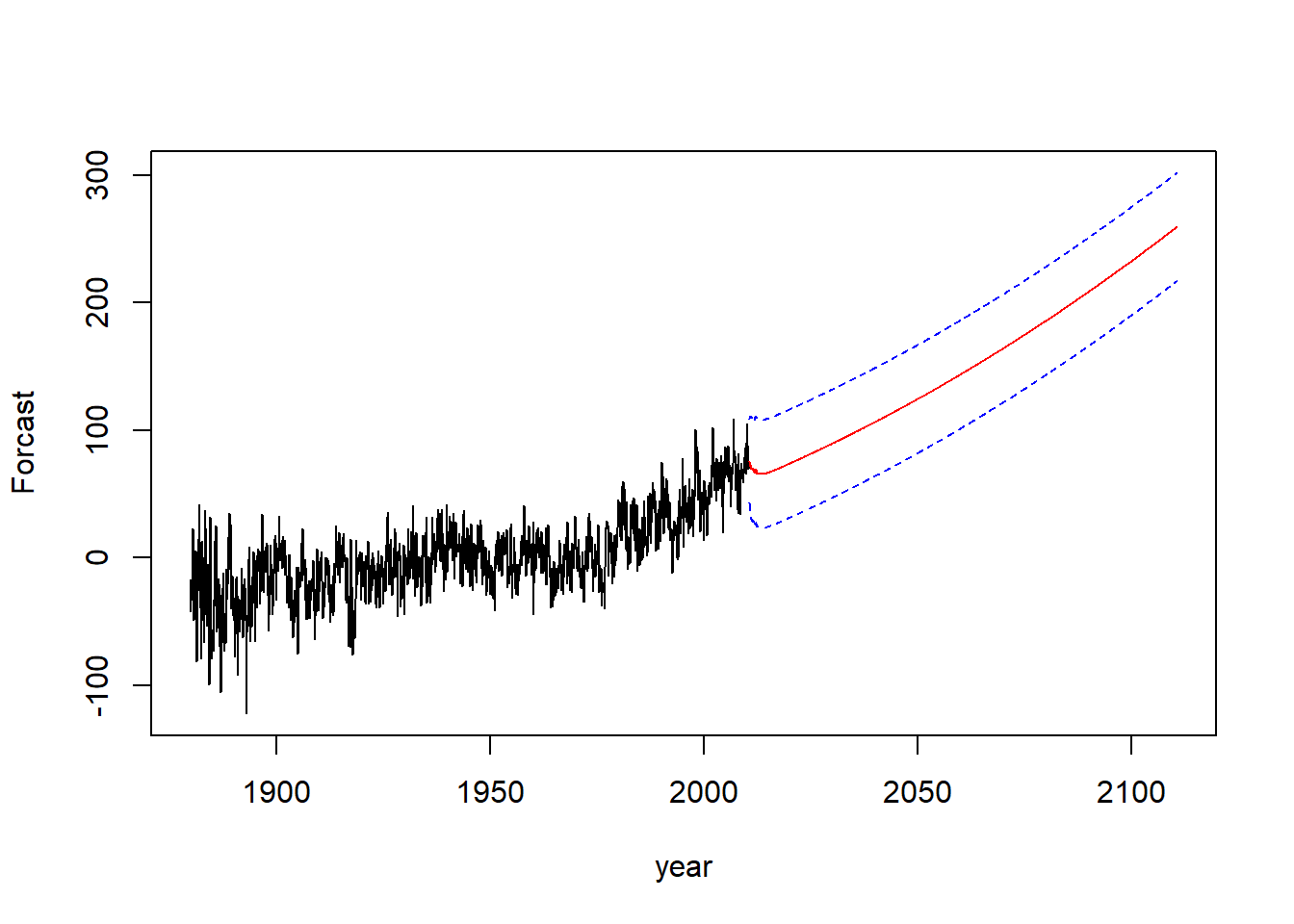
图16.20: 非随机二次趋势模型的100年长期预测
非随机二次多项式趋势的模型给出了一个二次多项式增长长期预测, 而且预测的区间长度略增长后就稳定不变。 预测方差最后趋于固定趋势回归的残差方差。
两个长期预测模型给出截然不同的结果, 也无法证明哪一个结果正确, 则两个结果都不能作为长期预测结果。
16.7 讨论
这个例子展示了如何从序列图、差分、ACF、PACF等发现可能的建模方向, 如何逐步改善模型, 随机趋势与非随机趋势的比较与各自的建模步骤, 如何比较模型,长期预报,等等。
下面对一些其他重要问题进行讨论。
16.7.1 模型的不确定性
所有的模型都是错误的, 只不过其中一部分是有用的。 模型是所分析过程的近似。
模型的不确定性一方面来自样本的随机性以及由此而来的参数估计的随机误差, 还来自于不同模型选择的不确定性。 统计推断时应尽可能考虑这些不确定性。 时间序列分析中模型的不确定性可以通过模型平均来对抗。 比如, 全球温度异常模型的短期预测可以用三个模型的预测的简单平均计算, 但也仅适用于短期预测。
16.7.2 短期预测与长期预测
目标是短期预测还是长期预测可能会影响模型选择, 甚至于超前一步预测最优的模型不一定是超前两步预测最优的。 文献中有自适应预测研究,见(Tiao and Tsay 1994)。
16.7.3 分段非随机趋势模型
从数据的时间序列图观察,在大约1980年以后斜率明显增加。 所以,设计一个斜率分为两段的模型:
\[ y_t = \beta_0 + (\beta_1 + \beta_2 I_t) t + \eta_t, \] 其中\(I_t\)为\(t > 1212\)的示性函数, 1212对应于1980年12月, 上述模型的回归斜率项在1980年12月之前为\(\beta_1\), 在1980年12月之后为\(\beta_1 + \beta_2\)。 令\(x_t = I_t t\),则模型可以写成 \[ y_t = \beta_0 + \beta_1 t + \beta_2 x_t + \eta_t . \]
tt <- seq(length(Gtemp))
xt <- ifelse(tt>1212, tt, 0)
resm <- arima(Gtemp, xreg=cbind(tt, xt), order=c(2,0,1))
resm
##
## Call:
## arima(x = Gtemp, order = c(2, 0, 1), xreg = cbind(tt, xt))
##
## Coefficients:
## ar1 ar2 ma1 intercept tt xt
## 1.1563 -0.2221 -0.7119 -29.0621 0.0313 0.0221
## s.e. 0.0716 0.0541 0.0627 4.0058 0.0056 0.0042
##
## sigma^2 estimated as 269.5: log likelihood = -6612.92, aic = 13239.83增加季节项:
tt <- seq(length(Gtemp))
xt <- ifelse(tt>1212, tt, 0)
resm <- arima(Gtemp, xreg=cbind(tt, xt), order=c(2,0,1),
              seasonal=list(order=c(0,0,2), period=12))
resm
##
## Call:
## arima(x = Gtemp, order = c(2, 0, 1), seasonal = list(order = c(0, 0, 2), period = 12),
## xreg = cbind(tt, xt))
##
## Coefficients:
## ar1 ar2 ma1 sma1 sma2 intercept tt xt
## 1.1168 -0.1940 -0.6788 0.0119 0.0820 -29.0241 0.0314 0.0220
## s.e. 0.0754 0.0556 0.0670 0.0263 0.0239 4.1381 0.0058 0.0044
##
## sigma^2 estimated as 267.4: log likelihood = -6606.89, aic = 13231.79删去不显著的Sma1项:
tt <- seq(length(Gtemp))
xt <- ifelse(tt>1212, tt, 0)
fixed <- rep(NA_real_, 8)
fixed[4] <- 0
mod7 <- arima(Gtemp, xreg=cbind(tt, xt), order=c(2,0,1),
              seasonal=list(order=c(0,0,2), period=12),
              fixed=fixed)
mod7
##
## Call:
## arima(x = Gtemp, order = c(2, 0, 1), seasonal = list(order = c(0, 0, 2), period = 12),
## xreg = cbind(tt, xt), fixed = fixed)
##
## Coefficients:
## ar1 ar2 ma1 sma1 sma2 intercept tt xt
## 1.1220 -0.1973 -0.6835 0 0.0823 -29.2630 0.0317 0.0219
## s.e. 0.0727 0.0542 0.0643 0 0.0239 4.1411 0.0058 0.0044
##
## sigma^2 estimated as 267.5: log likelihood = -6607, aic = 13230这个模型的AIC是现有的模型中最好的。 从结果中xt自变量的估计值和标准误差比值看, 这一项是显著的,即认为\(\beta_2 \neq 0\), 说明分段是成立的。
残差诊断:

图16.21: 分段模型的残差诊断
##
##  Ljung-Box test
##
## data:  Residuals from ARIMA(2,0,1)(0,0,2)[12] with non-zero mean
## Q* = 30.932, df = 19, p-value = 0.04107
##
## Model df: 5.   Total lags used: 24
基本可以接受残差诊断结果。Ljung-Box白噪声诊断:
##
##  Box-Ljung test
##
## data:  mod7$residuals
## X-squared = 17.92, df = 12, p-value = 0.1181这个模型从1981年开始温度的月升高率为\((0.0317+0.0219)=0.0536\), 年升高率为0.6432,即每年增加\(0.006432\)度, 平均155年增加1摄氏度。
虽然这个模型的样本内比较AIC结果最好, 但是并不推荐这种做法, 因为过于追求样本内的拟合优度往往导致过度拟合, 在样本外预测反而变差。 既然斜率可以变化, 那么未来斜率也可以变化, 作长期预测时因为未来的斜率变化不可知所以也不能用来做长期预测。 这里因为增长率加大以后样本量少所以不再比较样本外预测。
16.7.4 其它的数据
前面所用的全球气温异常数据来自GISS。 其它数据来源的数据建模也应得到类似结果。 这里使用NCDC和NOAA的数据, 单位为摄氏度。
读入数据:
##
## ── Column specification ────────────────────────────────────────────────────────
## cols(
##   X1 = col_double(),
##   X2 = col_double(),
##   X3 = col_double()
## )建立与MC1类似的模型:
mod8 <- arima(Gtemp2, order=c(1,1,2),
              seasonal=list(order=c(0,0,2), period=12),
              fixed=c(NA, NA, NA, 0, NA))
mod8
##
## Call:
## arima(x = Gtemp2, order = c(1, 1, 2), seasonal = list(order = c(0, 0, 2), period = 12),
## fixed = c(NA, NA, NA, 0, NA))
##
## Coefficients:
## ar1 ma1 ma2 sma1 sma2
## 0.5817 -1.2414 0.2639 0 0.0854
## s.e. 0.0704 0.0827 0.0781 0 0.0243
##
## sigma^2 estimated as 0.0881: log likelihood = -321.11, aic = 652.21因为数据不同, 这里的AIC不能与前一数据的模型的AIC比较。
模型诊断:
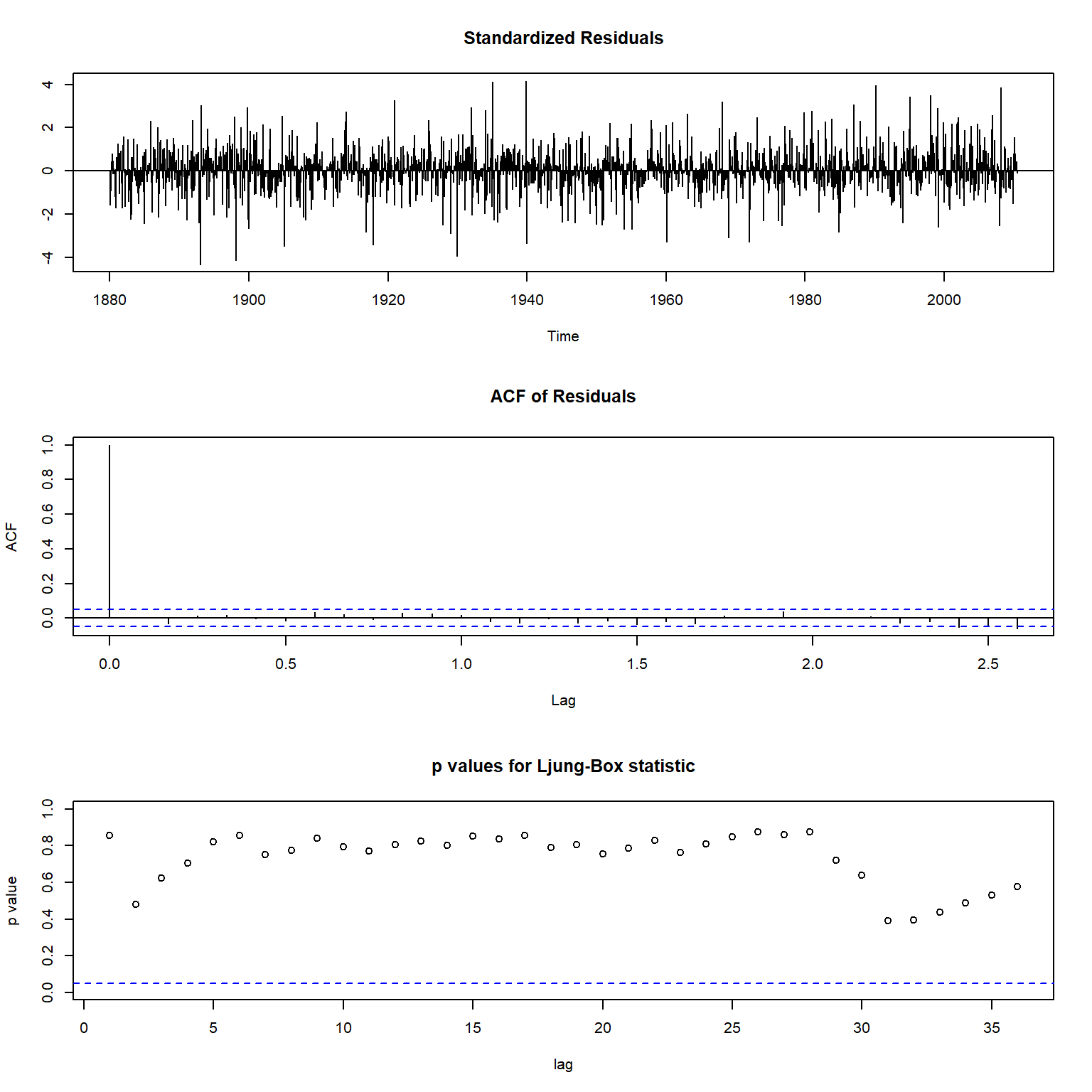
图16.22: 用NCDC和NOAA数据建立随机趋势模型的诊断
##
##  Ljung-Box test
##
## data:  Residuals from ARIMA(1,1,2)(0,0,2)[12]
## Q* = 17.88, df = 19, p-value = 0.5304
##
## Model df: 5.   Total lags used: 24
诊断说明模型是可取的。
样本外比较略。