15 线性时间序列案例学习—汽油价格
这一章用三个实例来详细讲解如何用R语言和线性时间序列模型分析实际数据, 并展现线性时间序列模型的适用性与局限性。
数据为:
- 1997-01-06到2010-09-27的美国普通汽油价格周数据;
- 1880年1月到2010年8月全球温度异常值的月度数据;
- 美国失业率月度数据,包括首次申领失业救济金人数的序列以及不包括的序列。
这些数据是持续更新的, 也反映了全球或美国经济的重要方面, 其建模问题有足够的代表性。
用时间序列分析或者统计方法建模时, 最常遇到的困难是如何选取一个适当的模型。 当数据之间的动态相依性很复杂时, 模型的形式难以确定; 当有多个模型都表现很好时, 模型难以选择。
George Box教授关于建模问题有一句名言(G. E. P. Box 1976):
所有的模型都是错误的,但是其中有一些是有用的。
不同的研究目的可能偏向于不同的模型。
时间序列数据建模的一些指导原则:
- 数据仅是可利用信息的一部分, 专业知识、常识、历史事件等都是需要考虑的可利用信息。
- 多个模型可能表现相近, 这时并没有一个“正确的”模型, 选择一个就可以。
- 在预测时,可以结合多个模型来改善预测效果。
- 建模的过程是从最简单的模型到逐步复杂, 千万不能以为理论上越复杂、理解和掌握的人数越少的模型才是越好的模型。
- 模型应尽可能选择更简洁的模型, 如果两个模型的表现相近, 一定要选择更简单的一个。 这也是避免过度拟合的要求。 过度拟合会导致模型的外推预测能力丧失。
15.1 数据读入与探索性分析
原油价格和汽油价格对美国经济的重要影响:
- 20实际70年代初期石油危机展示了石油资源的战略意义。
- 2008年汽油价格高涨影响了居民生活:
- 交通成本上涨
- 供热成本上涨
- 食品,服务价格上涨==> 通货膨胀
- 降低了消费者在其它消费项目上的可支配收入,可能导致经济萧条
研究美国汽油价格以及原油价格对其影响。 数据为美国普通石油价格周数据,从1997-01-06到2010-09-27。 时间是每周三, 共717个时间点; 美国原油价格周数据,从1997-01-03到2010-09-24。 时间是每周日。共717个时间点。 原油价格比汽油价格早3天发布。
读入数据:石油价格和汽油价格分成了两个输入文件。
石油价格的输入文件w-petroprice.txt又是一个用单个空格、多个空格、制表符、空格加制表符分隔的文件。
这种文件千万不要自己制造出来。
目前readr包还不支持这样的文件,
用R原来的read.table()函数来读入:
da1 <- read.table(
  "w-petroprice.txt", header=TRUE)
xts.petrol <- xts(
  da1[,-(1:3)], make_date(da1[["Year"]], da1[["Mon"]], da1[["Day"]]))
da2 <- read_table(
  "w-gasoline.txt", col_names="pgas",
  col_types=cols(.default=col_double())
)
xts.gasoline <- xts(da2[[1]], index(xts.petrol)+3)
xts.pgs <- log(xts.gasoline[,1]) # 美国普通汽油价格对数值序列
pgs <- coredata(xts.pgs)[,1]
xts.pus <- log(xts.petrol[,"US"]) # 美国原油价格对数值序列
pus <- coredata(xts.pus)[,1]
## 一阶差分序列
dpgs <- diff(pgs)
dpus <- diff(pus)
如果希望用readr包来读入, 最简单的解决办法是用文本编辑器编辑,将制表符都替换成单个空格; 下面的R程序用了R语言的文件操作和正则表达式进行替换:
la <- readLines("w-petroprice.txt")
la <- gsub("\\s+", " ", la)
la <- gsub("^\\s+|\\s$", "", la)
da1 <- read_table(
  paste(la, collapse="\n"),
  col_types=cols(.default=col_double())
)
汽油价格对数值的时间序列图:
plot(
  xts.pgs,
  main="ln Gasoline Price",
  major.ticks="years", minor.ticks=NULL,
  grid.ticks.on="years",
  col="red"
)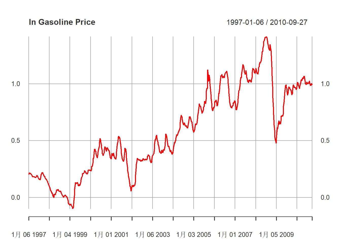
图15.1: 汽油价格对数值序列
原油价格对数值的时间序列图:
plot(
  xts.pus,
  main="ln Petrol Price",
  major.ticks="years", minor.ticks=NULL,
  grid.ticks.on="years",
  col="black"
)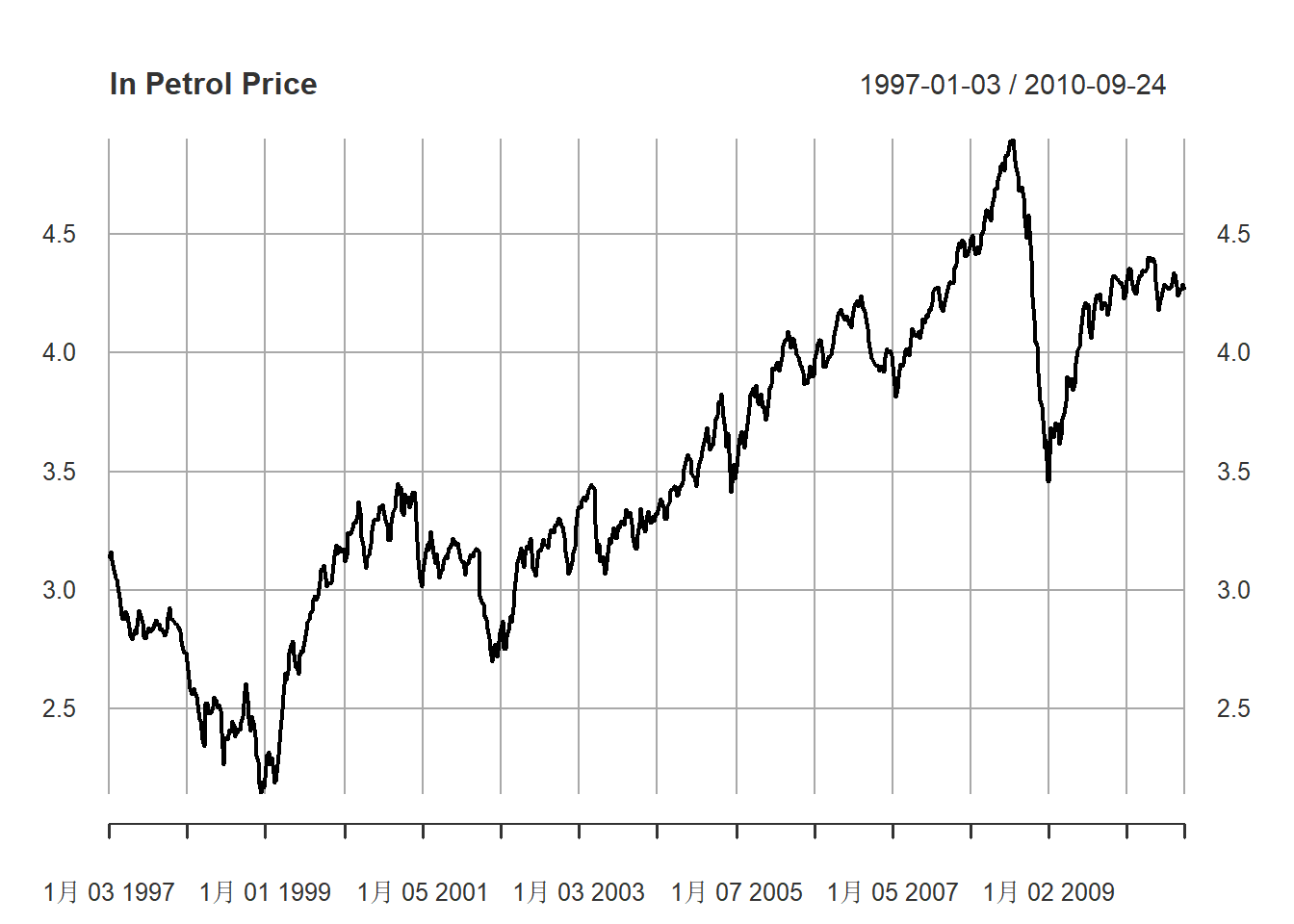
图15.2: 原油价格对数值序列
将对数汽油价格与对数原油价格同时绘制:
xts.pgs.pus <- xts(cbind(pgs, pus), index(xts.pgs))
plot(
  xts.pgs.pus,
  main="ln Petrol Price and ln Gasoline Price",
  major.ticks="years", minor.ticks=NULL,
  grid.ticks.on="years",
  col=c("red", "black")
)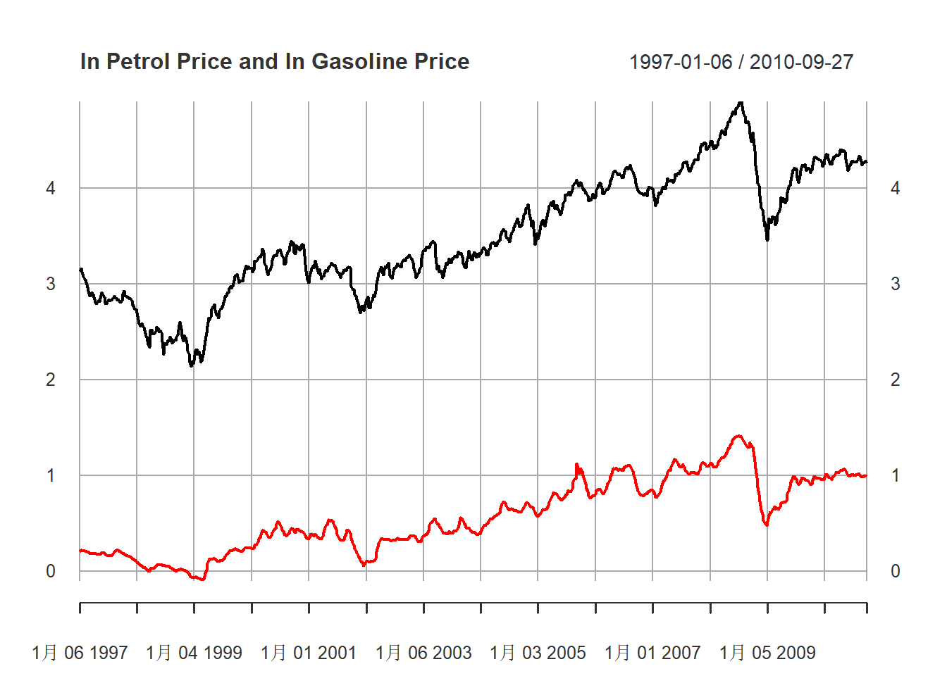
图15.3: 汽油、原油价格对数值序列
为什么要用对数价格而不用原始价格? 请看原始价格的图形:
xts.orig.pgs.pus <- xts(cbind(exp(pgs), exp(pus)), index(xts.pgs))
plot(
  xts.orig.pgs.pus,
  main="Petrol Price and Gasoline Price",
  major.ticks="years", minor.ticks=NULL,
  grid.ticks.on="years",
  col=c("red", "black")
)
图15.4: 汽油、原油价格原始序列
从图形可以看出, 原始价格随时间而振幅变大, 两个序列画在同一序列很难看出有同步变化。 对数变换是最常见的克服指数增长、将比例关系转换成线性关系的变换。
对数汽油价格对对数原油价格的散点图:
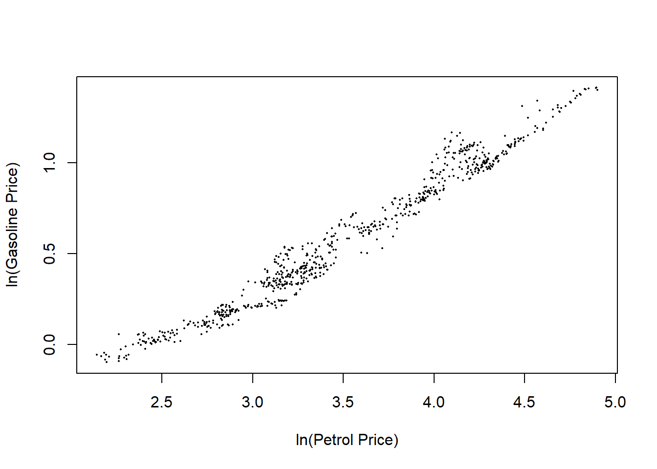
图15.5: 对数汽油对对数原油价格
可以看出汽油价格与同期原油价格相关性很强,相关系数为:
##
##  Pearson's product-moment correlation
##
## data:  pus and pgs
## t = 143.56, df = 715, p-value < 2.2e-16
## alternative hypothesis: true correlation is not equal to 0
## 95 percent confidence interval:
##  0.9804472 0.9853826
## sample estimates:
##       cor
## 0.9830925
相关系数为0.98。
因为对数价格呈现出缓慢增长随机趋势, 所以使用其差分值(价格的对数变化率)作为建模数据。
汽油价格对数增长率的时间序列图:
plot(
  diff(xts.pgs),
  main="Gasoline Price Log Increase Rate",
  major.ticks="years", minor.ticks=NULL,
  grid.ticks.on="years",
  col="red"
)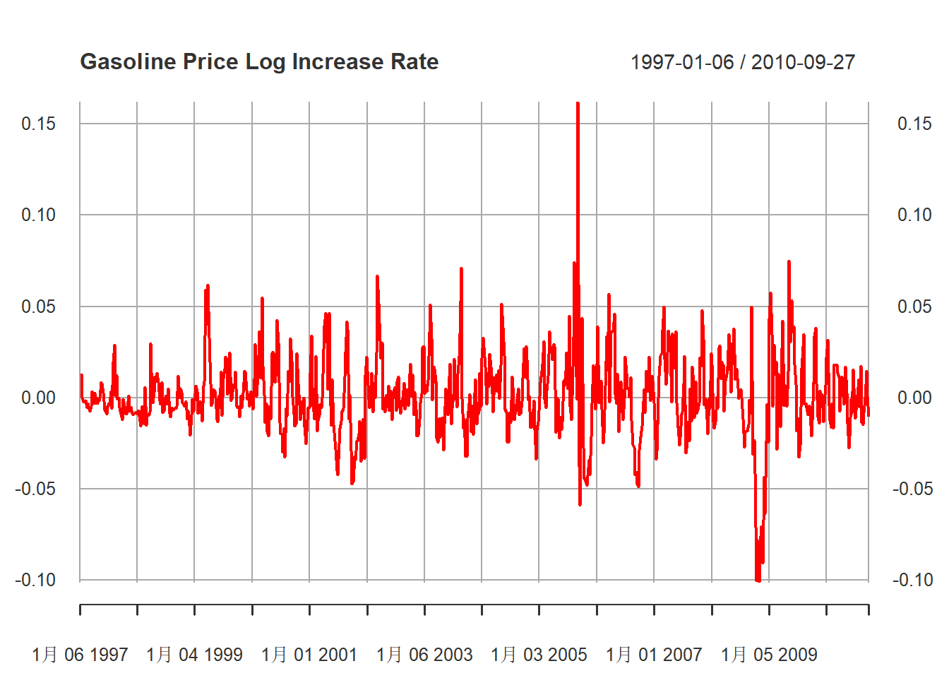
图15.6: 汽油价格对数增长率序列
汽油价格对数增长率的直方图:
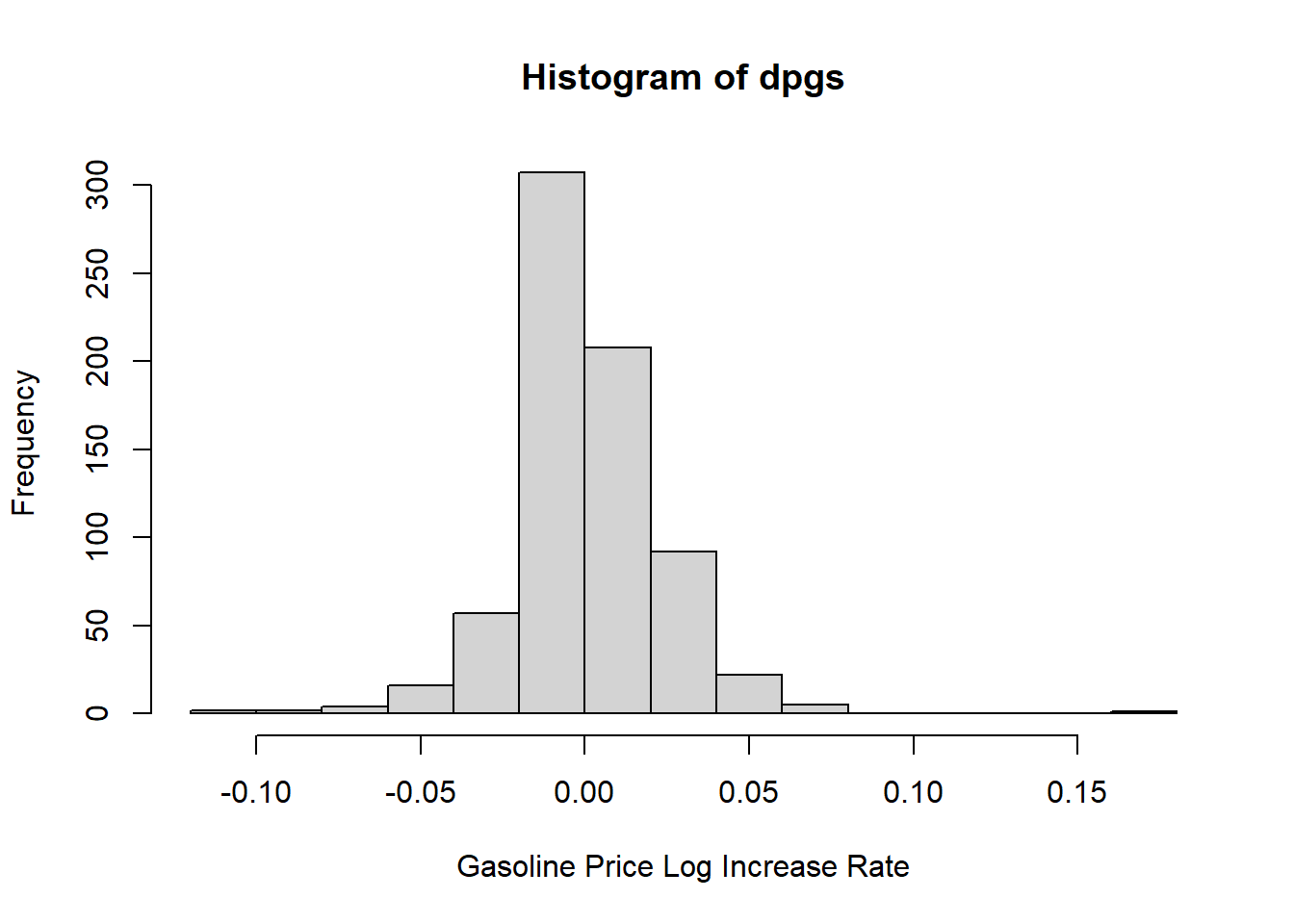
图15.7: 汽油价格对数增长率分布
汽油价格对数增长率的ACF:
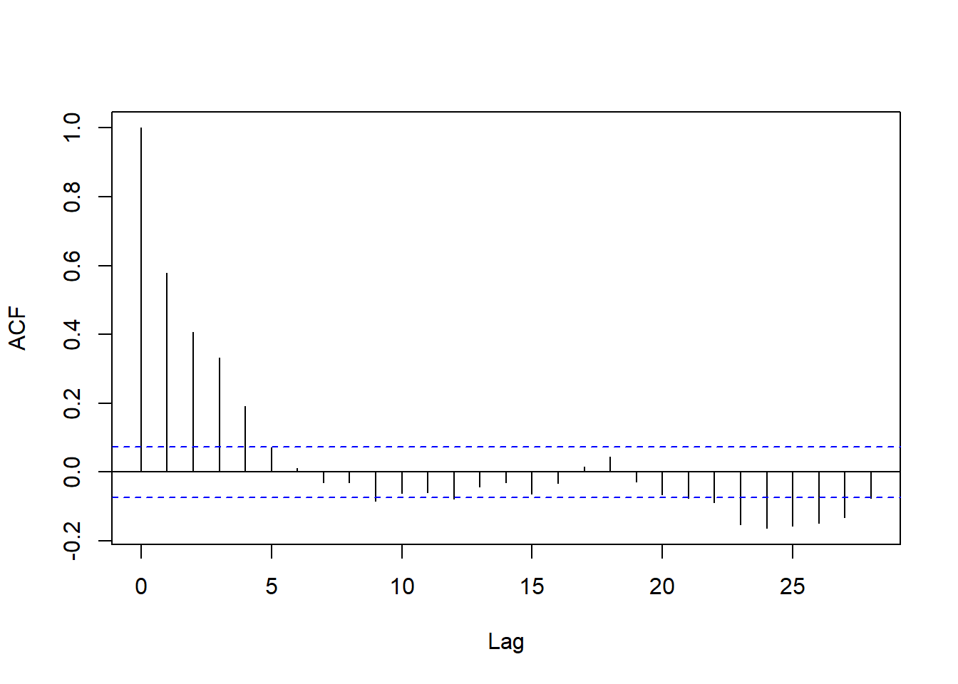
图15.8: 汽油价格对数增长率ACF
明显非白噪声,也不是低阶MA的典型形状。 ACF衰减很快,符合线性时间序列要求。
汽油价格对数增长率的PACF:
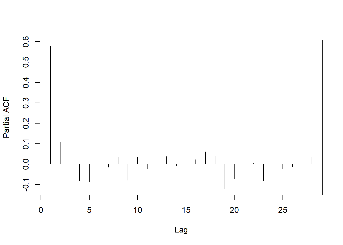
图15.9: 汽油价格对数增长率PACF
PACF在滞后1到5都是显著的,在滞后19处也比较显著。 用低阶AR有一定合理性。 PACF衰减很快,符合线性时间序列要求。
对数汽油价格序列的单位根检验:
##
## Title:
##  Augmented Dickey-Fuller Test
##
## Test Results:
##   PARAMETER:
##     Lag Order: 5
##   STATISTIC:
##     Dickey-Fuller: -1.5863
##   P VALUE:
##     0.4678
##
## Description:
##  Tue May 21 15:20:59 2024 by user: Lenovo
检验结果是有单位根。 但是, 如果扣除一个非随机线性趋势项检验,就没有单位根:
##
## Title:
##  Augmented Dickey-Fuller Test
##
## Test Results:
##   PARAMETER:
##     Lag Order: 5
##   STATISTIC:
##     Dickey-Fuller: -3.7307
##   P VALUE:
##     0.02246
##
## Description:
##  Tue May 21 15:20:59 2024 by user: Lenovo
下面还是按照对数汽油价格是单位根序列来建模。
15.2 AR(5)模型
记汽油价格对数增长率为\(x_t\)。 从时间序列图15.6来看, \(x_t\)在2005年有一个高涨:
plot(
  diff(xts.pgs)["2005"],
  main="Gasoline Price Log Increase Rate",
  major.ticks="month", minor.ticks=NULL,
  grid.ticks.on="months",
  col="red"
)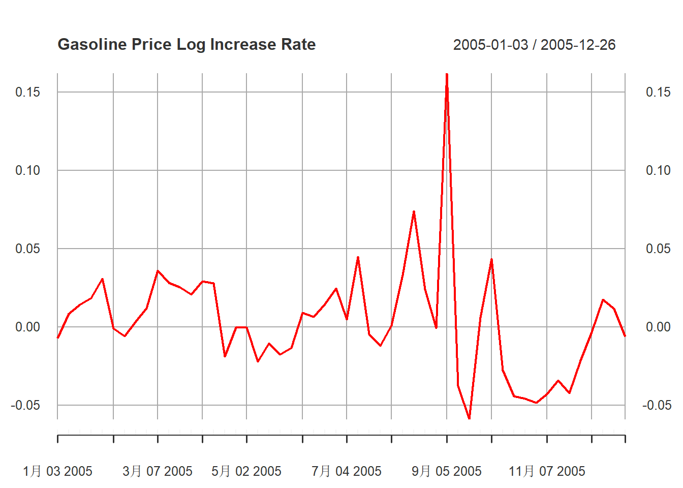
图15.10: 汽油价格对数增长率序列2005年
在2008年有一个大跌:
plot(
  diff(xts.pgs)["2008"],
  main="Gasoline Price Log Increase Rate",
  major.ticks="month", minor.ticks=NULL,
  grid.ticks.on="months",
  col="red"
)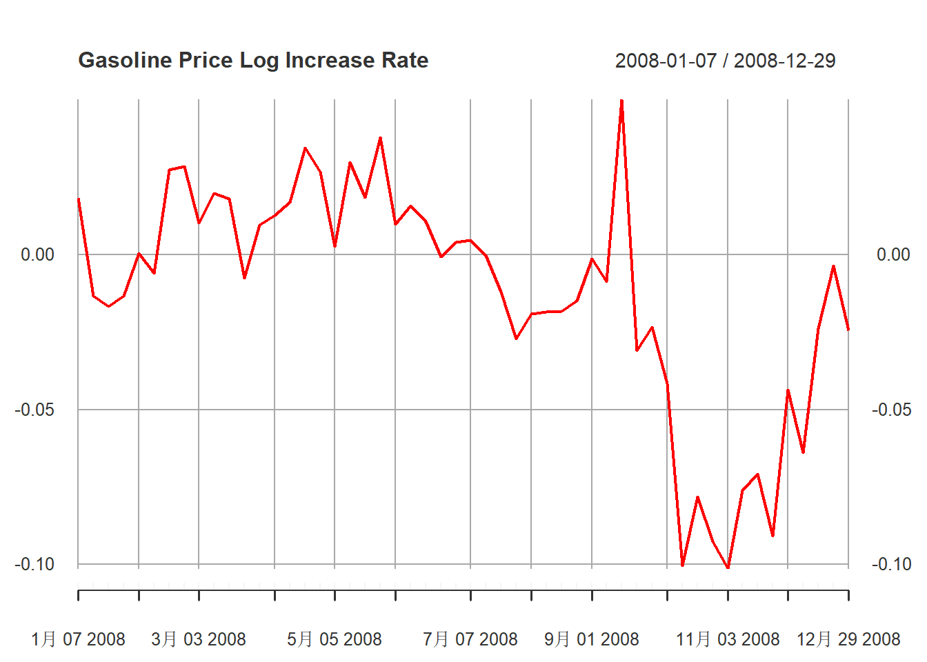
图15.11: 汽油价格对数增长率序列2008年
这些极端值为建模增加了困难。
从\(x_t\)的ACF和PACF来看, 都是快速衰减, 比较符合线性时间序列特征。
使用AIC对AR模型定阶:
##
## Call:
## ar(x = dpgs, method = "mle")
##
## Coefficients:
##       1        2        3        4        5
##  0.5068   0.0786   0.1352  -0.0362  -0.0869
##
## Order selected 5  sigma^2 estimated as  0.000326
AIC选择5阶, 这也与PACF的观察结果吻合。
先建立一个含有常数项的AR(5)模型, 再考虑常数项是否需要:
##
## Call:
## arima(x = dpgs, order = c(5, 0, 0), include.mean = TRUE)
##
## Coefficients:
##          ar1     ar2     ar3      ar4      ar5  intercept
##       0.5067  0.0786  0.1352  -0.0362  -0.0867     0.0011
## s.e.  0.0372  0.0417  0.0415   0.0417   0.0372     0.0017
##
## sigma^2 estimated as 0.000326:  log likelihood = 1858.07,  aic = -3702.14
从intercept的估计值与SE的比较来看, 均值是不显著的。 (如果估计值落入正负二倍SE范围就不显著)。 所以改为一个不含常数项的AR(5)模型:
##
## Call:
## arima(x = dpgs, order = c(5, 0, 0), include.mean = FALSE)
##
## Coefficients:
##          ar1     ar2     ar3      ar4      ar5
##       0.5073  0.0788  0.1355  -0.0360  -0.0862
## s.e.  0.0372  0.0417  0.0415   0.0417   0.0372
##
## sigma^2 estimated as 0.0003262:  log likelihood = 1857.85,  aic = -3703.71
以上模型为 \[ x_t = 0.5073 x_{t-1} + 0.0788 x_{t-2} + 0.1355 x_{t-3} - 0.0360 x_{t-4} - 0.0862 x_{t-5} + \varepsilon_t, \ \text{Var}(\varepsilon_t) = 0.0003262 \]
逐个看AR系数的显著性, 可以发现ar4明显地不显著, ar2也接近于不显著。 删除第4个AR系数:
## Warning in arima(dpgs, order = c(5, 0, 0), fixed = c(NA, NA, NA, 0, NA), : some
## AR parameters were fixed: setting transform.pars = FALSE
##
## Call:
## arima(x = dpgs, order = c(5, 0, 0), include.mean = FALSE, fixed = c(NA, NA,
## NA, 0, NA))
##
## Coefficients:
## ar1 ar2 ar3 ar4 ar5
## 0.5036 0.0789 0.1220 0 -0.1009
## s.e. 0.0370 0.0418 0.0385 0 0.0330
##
## sigma^2 estimated as 0.0003265: log likelihood = 1857.48, aic = -3704.96修改后AIC值略有降低。
这样限制稀疏模型有可能破坏稳定性条件,所以用polyroot()函数求特征根,
看是否都在单位圆外:
## [1] 1.420831 1.606426 1.606426 1.420831 1.901977特征根都在单位圆外且距离单位圆较远, 说明线性时间序列模型是合适的。
如果进一步去掉滞后2系数:
## Warning in arima(dpgs, order = c(5, 0, 0), fixed = c(NA, 0, NA, 0, NA), : some
## AR parameters were fixed: setting transform.pars = FALSE
##
## Call:
## arima(x = dpgs, order = c(5, 0, 0), include.mean = FALSE, fixed = c(NA, 0, NA,
## 0, NA))
##
## Coefficients:
## ar1 ar2 ar3 ar4 ar5
## 0.5360 0 0.1513 0 -0.0930
## s.e. 0.0329 0 0.0354 0 0.0328
##
## sigma^2 estimated as 0.0003281: log likelihood = 1855.7, aic = -3703.4AIC值比仅去掉滞后4的模型变大了。 所以应选择仅去掉滞后4的系数。
限制\(\phi_4=0\)的AR(5)模型为: \[ x_t = 0.5036 x_{t-1} + 0.0789 x_{t-2} + 0.1220 x_{t-3} - 0.1009 x_{t-5} + \varepsilon_t, \ \text{Var}(\varepsilon_t) = 0.0003265 \]
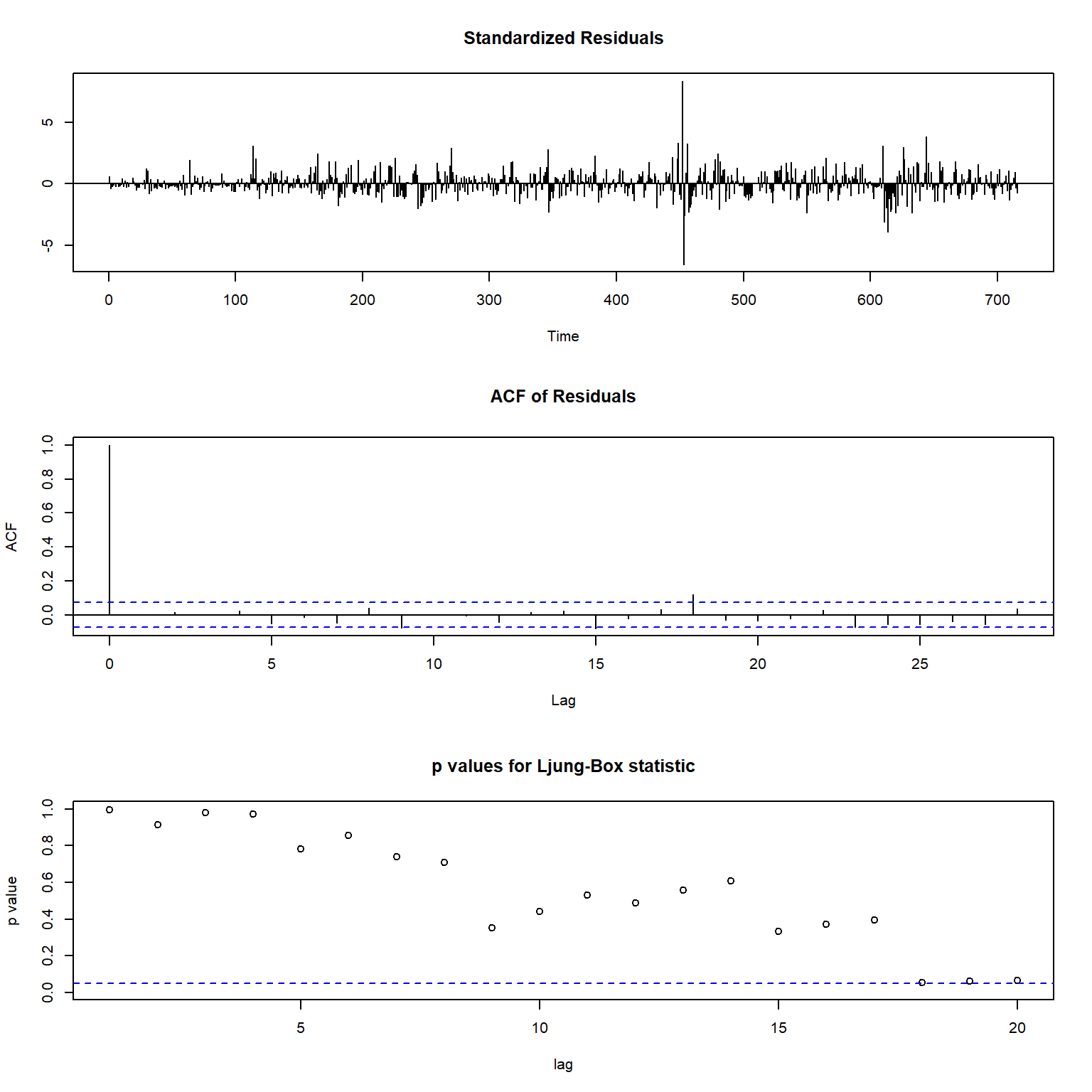
称此模型为候选模型1(MC1)。 对此模型做诊断图:
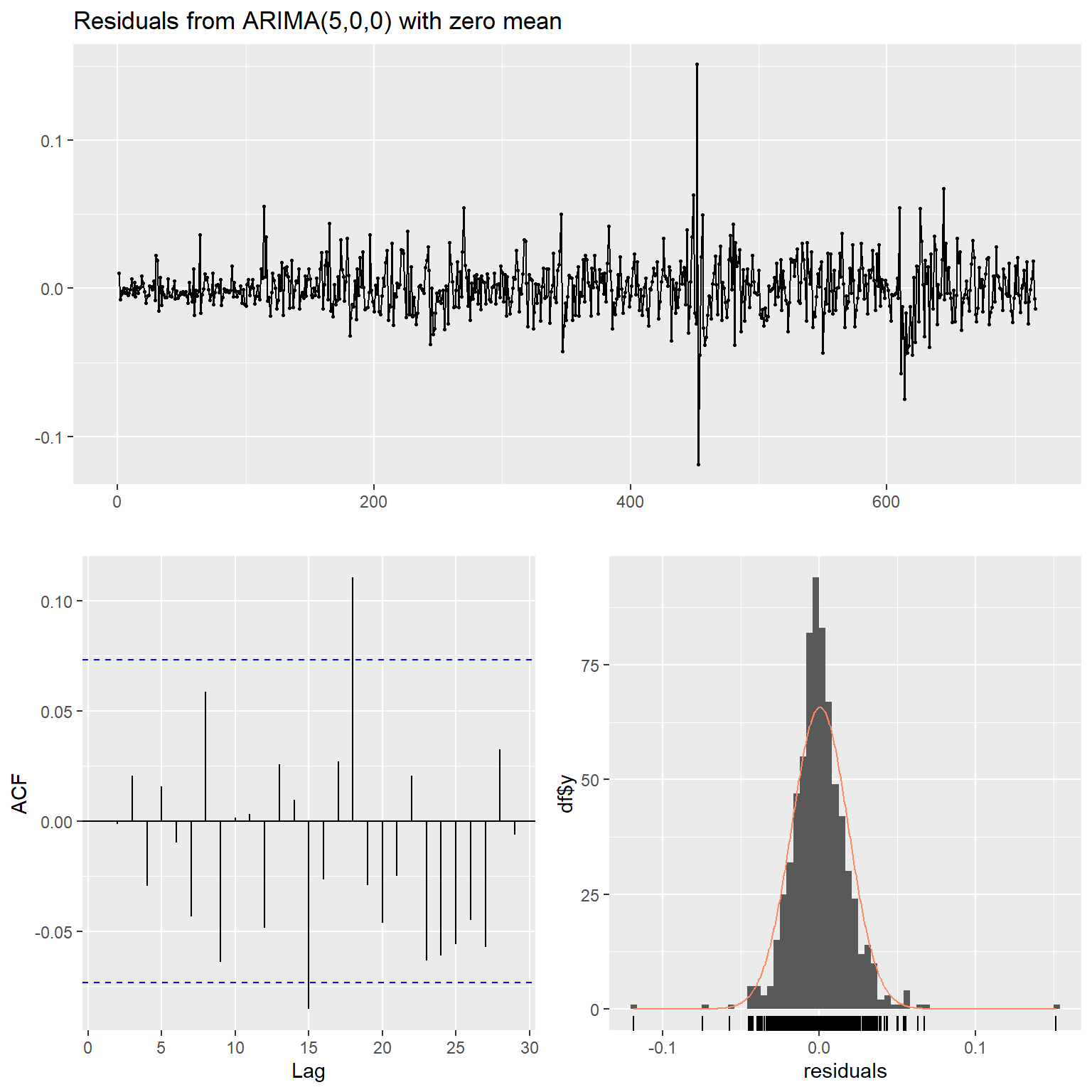
图15.12: 候选模型1诊断
##
##  Ljung-Box test
##
## data:  Residuals from ARIMA(5,0,0) with zero mean
## Q* = 7.997, df = 5, p-value = 0.1564
##
## Model df: 5.   Total lags used: 10
从诊断图看,标准化残差仍有较大的异常值。 ACF已经基本符合白噪声要求。 白噪声检验通过。 这些诊断支持了候选模型1。
15.3 ARMA(1,3)模型
考虑汽油价格序列对数增长率的其它线性时间序列模型。 注意到PACF中滞后1最显著,其它显著位置是刚刚超出0.05水平界限。 所以考虑用AR(1); 但是,因为ACF和PACF并不在低阶截尾, 所以单用AR或者单用MA可能不够, 尝试用ARMA。
先看AR(1)的表现:
resm6 <- arima(
  dpgs, order=c(1,0,0),
  include.mean=FALSE)
forecast::Acf(residuals(resm6), lag.max=10, main="")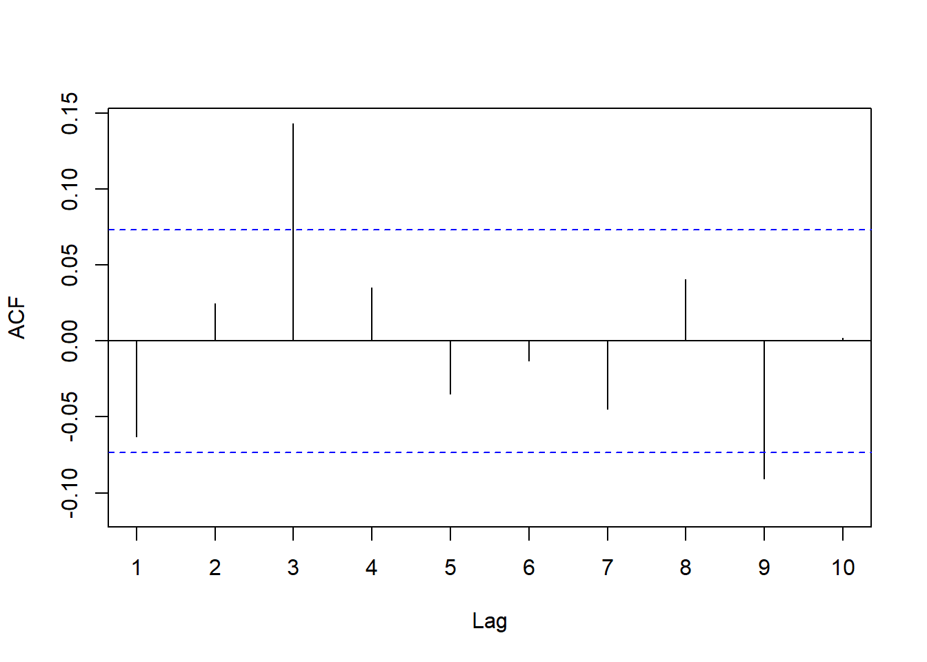
图15.13: AR(1)的残差ACF
AR(1)的ACF在滞后3有一个显著非零。尝试ARMA(1,3):
##
## Call:
## arima(x = dpgs, order = c(1, 0, 3), include.mean = FALSE)
##
## Coefficients:
##          ar1      ma1     ma2     ma3
##       0.5917  -0.0919  0.0413  0.1547
## s.e.  0.0750   0.0774  0.0489  0.0435
##
## sigma^2 estimated as 0.0003273:  log likelihood = 1856.65,  aic = -3703.29
从系数估计值与SE的比较可以看出MA的系数1、系数2都不显著。 先去掉MA系数2, 拟合稀疏系数模型:
##
## Call:
## arima(x = dpgs, order = c(1, 0, 3), include.mean = FALSE, fixed = c(NA, NA,
##     0, NA))
##
## Coefficients:
##          ar1      ma1  ma2     ma3
##       0.6332  -0.1266    0  0.1411
## s.e.  0.0507   0.0595    0  0.0408
##
## sigma^2 estimated as 0.0003276:  log likelihood = 1856.3,  aic = -3704.6
这个模型的AIC比候选模型1略差一点。 MA系数1显著性在两可之间, 所以不继续精简。 模型为 \[ x_t = 0.6332 x_{t-1} + \varepsilon_t - 0.1266 \varepsilon_{t-1} + 0.1411 \varepsilon_{t-3}, \ \text{Var}(\varepsilon_t) = 0.0003276 \] 称此模型为候选模型2(MC2)。
对候选模型2作诊断图:
##
##  Ljung-Box test
##
## data:  Residuals from ARIMA(1,0,3) with zero mean
## Q* = 9.9702, df = 6, p-value = 0.1259
##
## Model df: 4.   Total lags used: 10
标准化残差图仍有大异常值。 ACF已经符合白噪声表现; Ljung-Box白噪声检验基本符合白噪声要求。
因为候选模型1和候选模型2是类似的模型, 候选模型1的AIC较优, 所以两者相比选择候选模型1。
15.4 固定线性趋势模型
考虑用非随机线性趋势对汽油价格对数值序列建模。
##
## Call:
## lm(formula = pgs ~ tmp.t)
##
## Residuals:
##      Min       1Q   Median       3Q      Max
## -0.53400 -0.12170 -0.00928  0.12268  0.44298
##
## Coefficients:
##               Estimate Std. Error t value Pr(>|t|)
## (Intercept) -6.664e-03  1.276e-02  -0.522    0.602
## tmp.t        1.627e-03  3.079e-05  52.848   <2e-16 ***
## ---
## Signif. codes:  0 '***' 0.001 '**' 0.01 '*' 0.05 '.' 0.1 ' ' 1
##
## Residual standard error: 0.1707 on 715 degrees of freedom
## Multiple R-squared:  0.7962, Adjusted R-squared:  0.7959
## F-statistic:  2793 on 1 and 715 DF,  p-value: < 2.2e-16
回归结果显著。 考察残差序列:
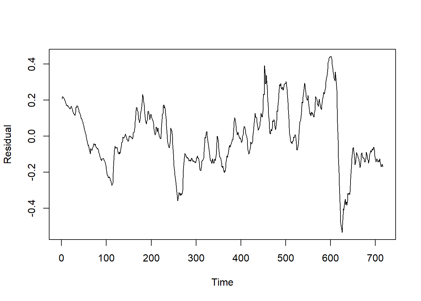
图15.14: 非随机线性趋势模型残差序列
序列呈现出一定的缓慢随机水平变化, 提示非平稳。 残差的ACF图:
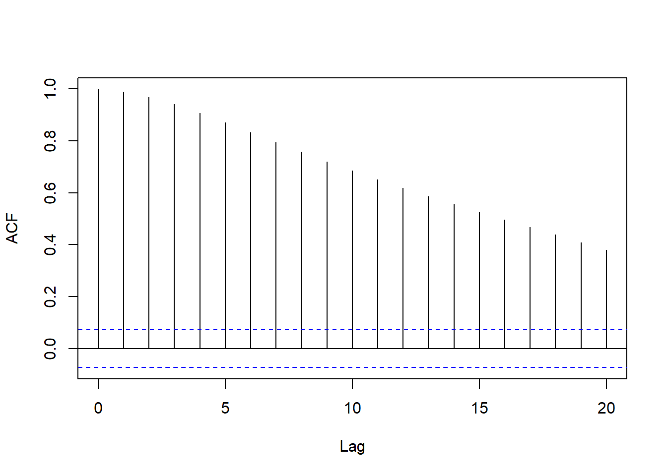
图15.15: 非随机线性趋势模型残差的ACF
说明残差序列的ACF是缓慢衰减的, 不太适用线性时间序列加非随机线性趋势作为模型。
15.5 引入石油价格解释变量的模型
考虑用石油价格对数值作为解释变量, 对汽油价格对数值序列建模。 设\(\{x_t \}\)为汽油价格对数增长率, \(\{ z_t \}\)为原油价格对数增长率, 使用带有误差自相关的回归模型。
先做简单回归:
\[ x_t = a + b z_t + \varepsilon_t \]
##
## Call:
## lm(formula = dpgs ~ dpus)
##
## Residuals:
##       Min        1Q    Median        3Q       Max
## -0.076840 -0.009456 -0.000279  0.008804  0.150721
##
## Coefficients:
##              Estimate Std. Error t value Pr(>|t|)
## (Intercept) 0.0006472  0.0006876   0.941    0.347
## dpus        0.2865347  0.0150791  19.002   <2e-16 ***
## ---
## Signif. codes:  0 '***' 0.001 '**' 0.01 '*' 0.05 '.' 0.1 ' ' 1
##
## Residual standard error: 0.01839 on 714 degrees of freedom
## Multiple R-squared:  0.3359, Adjusted R-squared:  0.3349
## F-statistic: 361.1 on 1 and 714 DF,  p-value: < 2.2e-16
可以看出截距项不显著。 尽管因为残差可能有自相关使得检验不一定精确, 因为两个序列都是差分序列,原始序列相关系数很大, 所以回归模型没有常数项是正常的。 将上述回归模型改为不带截距项的模型:
\[ x_t = b z_t + \varepsilon_t \]
##
## Call:
## lm(formula = dpgs ~ -1 + dpus)
##
## Residuals:
##       Min        1Q    Median        3Q       Max
## -0.076149 -0.008834  0.000365  0.009441  0.151350
##
## Coefficients:
##      Estimate Std. Error t value Pr(>|t|)
## dpus  0.28703    0.01507   19.05   <2e-16 ***
## ---
## Signif. codes:  0 '***' 0.001 '**' 0.01 '*' 0.05 '.' 0.1 ' ' 1
##
## Residual standard error: 0.01839 on 715 degrees of freedom
## Multiple R-squared:  0.3366, Adjusted R-squared:  0.3357
## F-statistic: 362.8 on 1 and 715 DF,  p-value: < 2.2e-16
查看回归残差的ACF:
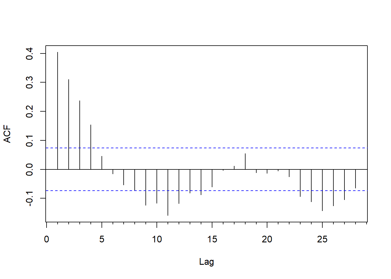
图15.16: 回归模型的残差序列的ACF
查看回归残差的PACF:
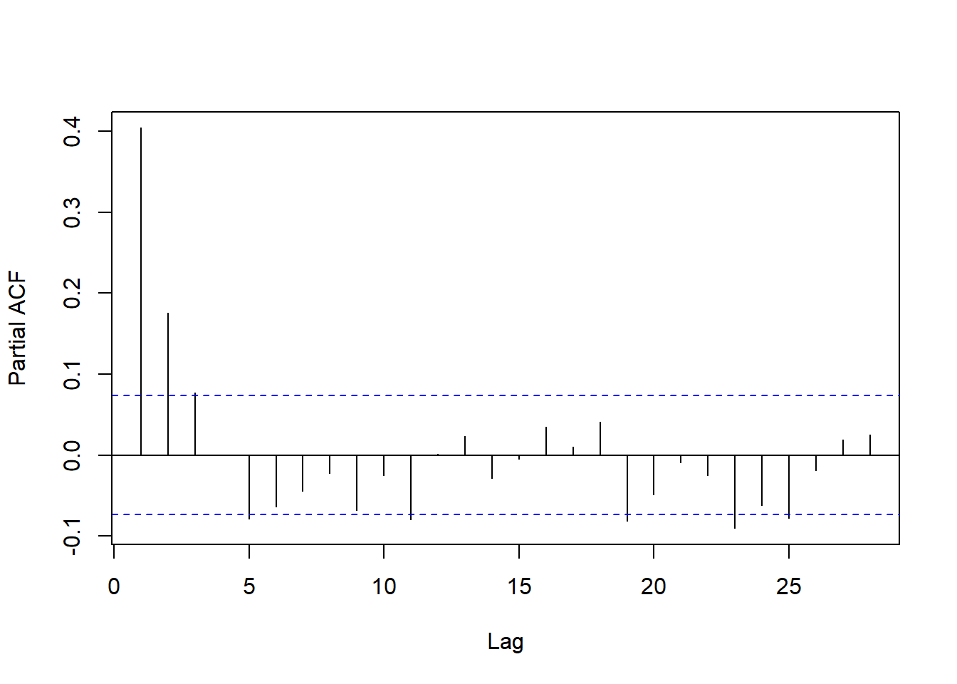
图15.17: 回归模型的残差序列的PACF
回归残差的ACF和PACF都是快速衰减的, 但都不截尾。 从PACF看, 基本在第5阶之后截尾了。
用AIC对残差的AR模型定阶:
##
## Call:
## ar(x = resm11$residuals, method = "mle")
##
## Coefficients:
##       1        2        3        4        5        6
##  0.3140   0.1575   0.0943   0.0346  -0.0568  -0.0625
##
## Order selected 6 sigma^2 estimated as 0.0002689AIC选择6阶。试用arima()函数估计AR(6):
##
## Call:
## arima(x = resm11$residuals, order = c(6, 0, 0))
##
## Coefficients:
##          ar1     ar2     ar3     ar4      ar5      ar6  intercept
##       0.3140  0.1576  0.0946  0.0353  -0.0582  -0.0631     0.0006
## s.e.  0.0372  0.0390  0.0394  0.0394   0.0390   0.0372     0.0012
##
## sigma^2 estimated as 0.0002689:  log likelihood = 1927.08,  aic = -3838.16
从估计结果看,均值(intercept)不显著, 滞后6系数不够显著, 滞后4系数不显著。 先拟合一个不带常数项的AR(5):
##
## Call:
## arima(x = resm11$residuals, order = c(5, 0, 0), include.mean = FALSE)
##
## Coefficients:
##          ar1     ar2     ar3     ar4      ar5
##       0.3193  0.1563  0.0891  0.0256  -0.0781
## s.e.  0.0372  0.0391  0.0394  0.0391   0.0372
##
## sigma^2 estimated as 0.0002701:  log likelihood = 1925.51,  aic = -3839.02
这个精简的模型的AIC实际上改善了。因为滞后4系数不显著,做一个稀疏系数AR(5):
## Warning in arima(resm11$residuals, order = c(5, 0, 0), fixed = c(NA, NA, : some
## AR parameters were fixed: setting transform.pars = FALSE##
## Call:
## arima(x = resm11$residuals, order = c(5, 0, 0), include.mean = FALSE, fixed = c(NA,
## NA, NA, 0, NA))
##
## Coefficients:
## ar1 ar2 ar3 ar4 ar5
## 0.3211 0.1592 0.0954 0 -0.0707
## s.e. 0.0371 0.0388 0.0382 0 0.0354
##
## sigma^2 estimated as 0.0002702: log likelihood = 1925.29, aic = -3840.59AIC继续有改善。 将外生回归变量加入模型中,直接建立带有自相关误差项的回归模型:
resm15 <- arima(
  dpgs, xreg=dpus, order=c(5,0,0), include.mean=FALSE,
  fixed=c(NA, NA, NA, 0, NA, NA))
## Warning in arima(dpgs, xreg = dpus, order = c(5, 0, 0), include.mean = FALSE, :
## some AR parameters were fixed: setting transform.pars = FALSE##
## Call:
## arima(x = dpgs, order = c(5, 0, 0), xreg = dpus, include.mean = FALSE, fixed = c(NA,
## NA, NA, 0, NA, NA))
##
## Coefficients:
## ar1 ar2 ar3 ar4 ar5 dpus
## 0.4037 0.1642 0.0961 0 -0.1014 0.1911
## s.e. 0.0386 0.0399 0.0386 0 0.0345 0.0136
##
## sigma^2 estimated as 0.0002532: log likelihood = 1948.48, aic = -3884.95这样建立的模型可以写成:
\[ \begin{aligned} x_t =& 0.1911 z_t + \xi_t, \\ \xi_t =& 0.4037 \xi_{t-1} + 0.1642 \xi_{t-2} + 0.0961 \xi_{t-3} - 0.1014 \xi_{t-5} + \varepsilon_t, \ \text{Var}(\varepsilon_t) = 0.0002532 \end{aligned} \]
称此模型为候选模型3(MC3)。 模型的诊断图形:
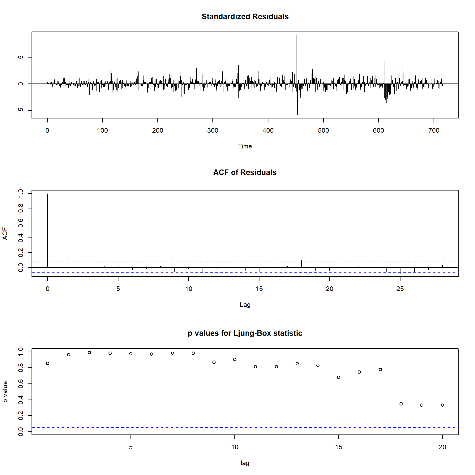
图15.18: 候选模型3的诊断图形
##
##  Ljung-Box test
##
## data:  Residuals from ARIMA(5,0,0) with zero mean
## Q* = 4.7748, df = 5, p-value = 0.444
##
## Model df: 5.   Total lags used: 10
从诊断图看,除了标准化残差还有大异常值以外, 残差的白噪声性质已经基本确认。 说明候选模型3是合适的。
将候选模型1与候选模型3进行比较。 这两个模型的比较是不公平的, 因为候选模型3利用了额外的原油价格信息。 候选模型1的残差方差估计是\(0.0003281\), AIC值是\(-3703.4\); 候选模型3的残差方差估计是\(0.0002532\), AIC值是\(-3884.95\)。 模型3的模型方差估计降低了23%, AIC也有明显改善。 后面可以看到模型3的预测效果也更好。
15.6 使用滞后石油价格解释变量的模型
数据中原油价格比汽油价格发布时间早3天, 这样, 利用回归模型预报时, 仅能超前1到3天预报, 超前4天时就没有对应的石油价格作为解释变量了。
考虑使用石油价格的前一个发布值作为解释变量, 这样石油价格比汽油价格提前10天。
简单回归模型:
\[ x_t = b z_{t-1} + \varepsilon_t \]
##
## Call:
## lm(formula = dpgs1 ~ -1 + dpus1)
##
## Residuals:
##       Min        1Q    Median        3Q       Max
## -0.088318 -0.011145 -0.000011  0.011391  0.161679
##
## Coefficients:
##       Estimate Std. Error t value Pr(>|t|)
## dpus1  0.18560    0.01716   10.81   <2e-16 ***
## ---
## Signif. codes:  0 '***' 0.001 '**' 0.01 '*' 0.05 '.' 0.1 ' ' 1
##
## Residual standard error: 0.02093 on 714 degrees of freedom
## Multiple R-squared:  0.1408, Adjusted R-squared:  0.1395
## F-statistic: 117 on 1 and 714 DF, p-value: < 2.2e-16注意这个回归\(R^2=0.14\)比间隔3天的回归的\(R^2=0.33\)小了许多, 预示着这个模型的预测效果远不如候选模型3。
对回归残差作ACF图:
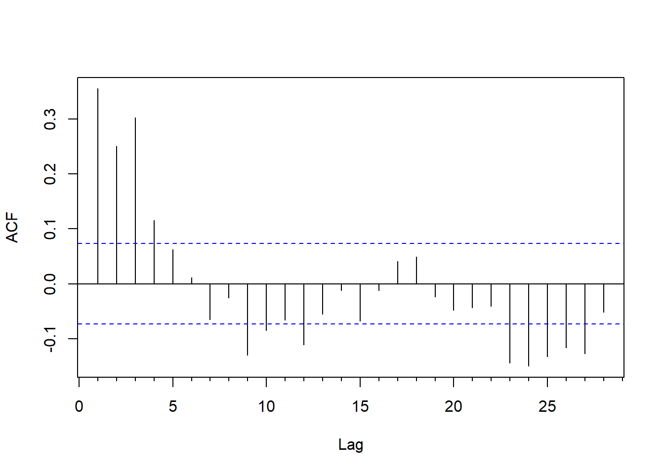
图15.19: 滞后回归的残差ACF
对回归残差作PACF图:
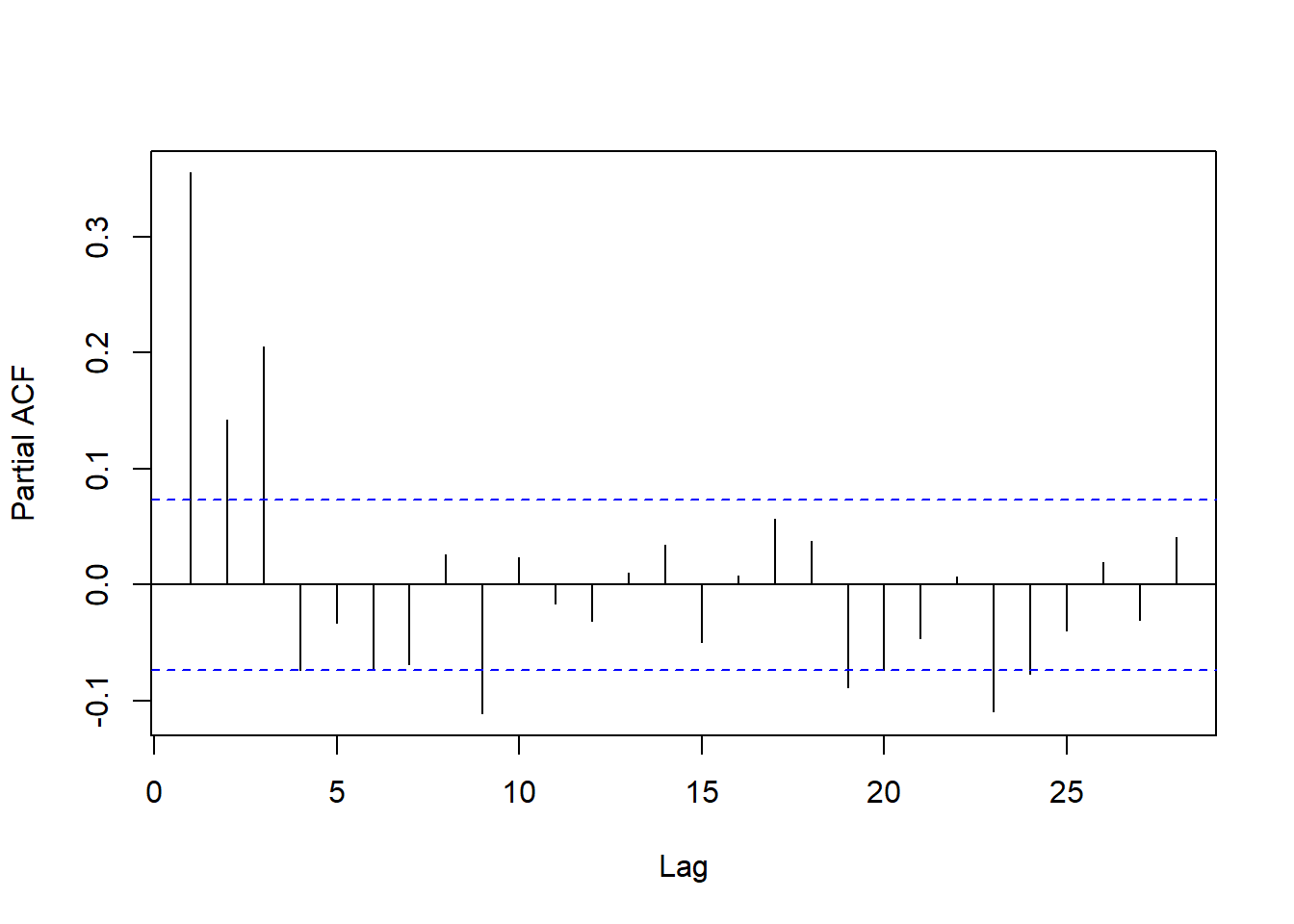
图15.20: 滞后回归的残差PACF
从残差的ACF和PACF看, 虽然都是快速衰减的, 但都不在低阶截尾。
用AIC为残差序列作AR定阶:
##
## Call:
## ar(x = resm16$residuals, method = "mle")
##
## Coefficients:
##       1        2        3        4        5        6        7        8
##  0.2851   0.0805   0.2343  -0.0411  -0.0169  -0.0284  -0.0652   0.0577
##       9
## -0.1101
##
## Order selected 9 sigma^2 estimated as 0.0003479选择9阶。用arima()估计:
##
## Call:
## arima(x = dpgs1, order = c(9, 0, 0), xreg = dpus1, include.mean = FALSE)
##
## Coefficients:
##          ar1     ar2     ar3      ar4      ar5      ar6      ar7     ar8
##       0.4559  0.0888  0.1679  -0.0468  -0.0653  -0.0195  -0.0362  0.0797
## s.e.  0.0425  0.0410  0.0423   0.0415   0.0416   0.0414   0.0410  0.0408
##           ar9   dpus1
##       -0.0882  0.0454
## s.e.   0.0373  0.0174
##
## sigma^2 estimated as 0.0003204:  log likelihood = 1861.55,  aic = -3701.1
查看各个系数的显著性, 用估计值除以标准误差得到检验统计量, 在等于零的零假设下近似服从标准正态分布:
arima.tstat <- function(mod) coef(mod)[coef(mod) != 0] / sqrt(diag(mod$var.coef))
round(sort(abs(arima.tstat(resm17))), 2)
## ar6 ar7 ar4 ar5 ar8 ar2 ar9 dpus1 ar3 ar1
## 0.47 0.88 1.13 1.57 1.95 2.16 2.36 2.61 3.97 10.73滞6, 7, 4, 5, 8的系数不显著。逐步进行改进,先去掉\(\phi_6\):
fixed <- rep(NA_real_, 10)
fixed[6] <- 0
resm18 <- arima(
  dpgs1, xreg=dpus1, include.mean=FALSE,
  order=c(9,0,0), fixed=fixed)
## Warning in arima(dpgs1, xreg = dpus1, include.mean = FALSE, order = c(9, : some
## AR parameters were fixed: setting transform.pars = FALSE##
## Call:
## arima(x = dpgs1, order = c(9, 0, 0), xreg = dpus1, include.mean = FALSE, fixed = fixed)
##
## Coefficients:
## ar1 ar2 ar3 ar4 ar5 ar6 ar7 ar8 ar9
## 0.4574 0.0889 0.1646 -0.0473 -0.0718 0 -0.0423 0.0794 -0.0908
## s.e. 0.0424 0.0410 0.0417 0.0415 0.0393 0 0.0389 0.0408 0.0369
## dpus1
## 0.0451
## s.e. 0.0174
##
## sigma^2 estimated as 0.0003205: log likelihood = 1861.44, aic = -3702.88## ar7 ar4 ar5 ar8 ar2 ar9 dpus1 ar3 ar1
## 1.09 1.14 1.83 1.95 2.17 2.46 2.60 3.95 10.78AIC有改进。再去掉\(\phi_7\):
fixed <- rep(NA_real_, 10)
fixed[c(6,7)] <- 0
resm19 <- arima(
  dpgs1, xreg=dpus1, include.mean=FALSE,
  order=c(9,0,0), fixed=fixed)
## Warning in arima(dpgs1, xreg = dpus1, include.mean = FALSE, order = c(9, : some
## AR parameters were fixed: setting transform.pars = FALSE##
## Call:
## arima(x = dpgs1, order = c(9, 0, 0), xreg = dpus1, include.mean = FALSE, fixed = fixed)
##
## Coefficients:
## ar1 ar2 ar3 ar4 ar5 ar6 ar7 ar8 ar9 dpus1
## 0.4618 0.0903 0.1617 -0.055 -0.078 0 0 0.0634 -0.0961 0.0431
## s.e. 0.0422 0.0411 0.0417 0.041 0.039 0 0 0.0381 0.0367 0.0172
##
## sigma^2 estimated as 0.0003211: log likelihood = 1860.85, aic = -3703.7## ar4 ar8 ar5 ar2 dpus1 ar9 ar3 ar1
## 1.34 1.66 2.00 2.20 2.50 2.62 3.87 10.94AIC有改进。再去掉\(\phi_4\):
fixed <- rep(NA_real_, 10)
fixed[c(6,7,4)] <- 0
resm20 <- arima(
  dpgs1, xreg=dpus1, include.mean=FALSE,
  order=c(9,0,0), fixed=fixed)
## Warning in arima(dpgs1, xreg = dpus1, include.mean = FALSE, order = c(9, : some
## AR parameters were fixed: setting transform.pars = FALSE##
## Call:
## arima(x = dpgs1, order = c(9, 0, 0), xreg = dpus1, include.mean = FALSE, fixed = fixed)
##
## Coefficients:
## ar1 ar2 ar3 ar4 ar5 ar6 ar7 ar8 ar9 dpus1
## 0.4580 0.0894 0.1414 0 -0.0989 0 0 0.0604 -0.0938 0.0403
## s.e. 0.0425 0.0412 0.0392 0 0.0358 0 0 0.0381 0.0367 0.0173
##
## sigma^2 estimated as 0.0003219: log likelihood = 1859.96, aic = -3703.91## ar8 ar2 dpus1 ar9 ar5 ar3 ar1
## 1.59 2.17 2.33 2.55 2.76 3.60 10.78AIC有改进。再去掉\(\phi_8\):
fixed <- rep(NA_real_, 10)
fixed[c(6,7,4,8)] <- 0
resm21 <- arima(
  dpgs1, xreg=dpus1, include.mean=FALSE,
  order=c(9,0,0), fixed=fixed)
## Warning in arima(dpgs1, xreg = dpus1, include.mean = FALSE, order = c(9, : some
## AR parameters were fixed: setting transform.pars = FALSE##
## Call:
## arima(x = dpgs1, order = c(9, 0, 0), xreg = dpus1, include.mean = FALSE, fixed = fixed)
##
## Coefficients:
## ar1 ar2 ar3 ar4 ar5 ar6 ar7 ar8 ar9 dpus1
## 0.4544 0.0877 0.1415 0 -0.0830 0 0 0 -0.0640 0.0406
## s.e. 0.0427 0.0413 0.0393 0 0.0345 0 0 0 0.0318 0.0176
##
## sigma^2 estimated as 0.000323: log likelihood = 1858.7, aic = -3703.4## ar9 ar2 dpus1 ar5 ar3 ar1
## 2.01 2.13 2.31 2.41 3.60 10.63AIC变差,所以退回到上一个模型,以AR(9)去掉滞后4、6、7系数的模型为候选模型4(MC4)。 注意,这个模型肯定不如模型3, 因为作为自变量的原油价格比汽油价格的发布时间早了10天。
15.7 样本外预测
下面比较MC1、MC3、MC4的样本外预测, 对最后的400个样本点作超前一步预测。 将这三个模型分别记为M1、M2、M3。
\[ \begin{aligned} M1:& x_t = \phi_1 x_{t-1} + \phi_2 x_{t-2} + \phi_3 x_{t-3} + \phi_5 x_{t-5} + \varepsilon_t \\ M2:& x_t = b z_t + \xi_t, \ \xi_t = \phi_1 \xi_{t-1} + \phi_2 \xi_{t-2} + \phi_3 \xi_{t-3} + \phi_5 \xi_{t-5} + \varepsilon_t \\ M3:& x_t = b z_{t-1} + \xi_t, \ \xi_t = \phi_1 \xi_{t-1} + \phi_2 \xi_{t-2} + \phi_3 \xi_{t-3} + \phi_5 \xi_{t-5} + \phi_8 \xi_{t-8} + \phi_9 \xi_{t-9} + \varepsilon_t \end{aligned} \]
为了统一起见,所有序列都放弃第一个观测。这样, 每个序列有715个观测, 对最后的400个做超前一步预测, 最初仅使用315个观测建模。
dpuslag1 <- dpus[-length(dpus)]
dpus1 <- dpus[-1]
dpgs1 <- dpgs[-1]
nmin <- 316
nmax <- length(dpgs1)
fcst <- matrix(NA_real_, nmax, 3)
fixed <- rep(NA_real_, 10)
fixed[c(4,6,7)] <- 0
for(t1 in nmin:nmax){
  # t1是要预测的时间点
  n <- t1-1 # 用来建模的序列长度
  # 利用1到n的样本建立三个模型
  m1 <- arima(dpgs1[1:n], order=c(5,0,0), include.mean=FALSE,
              fixed=c(NA, NA, NA, 0, NA), transform.pars=FALSE)
  m2 <- arima(dpgs1[1:n], xreg=dpus1[1:n],
              order=c(5,0,0), include.mean=FALSE,
              fixed=c(NA, NA, NA, 0, NA, NA), transform.pars=FALSE)
  m3 <- arima(dpgs1[1:n], xreg=dpuslag1[1:n],
              order=c(9,0,0), include.mean=FALSE,
              fixed=fixed, transform.pars=FALSE)

  # 分别获得超前一步预报
  fcst[t1,1] <- c(predict(m1, n.ahead=1, newxreg=NULL, se.fit=FALSE))
  fcst[t1,2] <- c(predict(m2, n.ahead=1, newxreg=dpus1[t1], se.fit=FALSE))
  fcst[t1,3] <- c(predict(m3, n.ahead=1, newxreg=dpuslag1[t1], se.fit=FALSE))
}
# 计算RMSFE和MAFE
rmsfe <- rep(0.0, 3)
mafe <- rep(0.0, 3)
for(j in 1:3){
  rmsfe[j] <- sqrt( mean((fcst[nmin:nmax, j] - dpgs1[nmin:nmax])^2) )
  mafe[j] <- mean(abs(fcst[nmin:nmax, j] - dpgs1[nmin:nmax]))
}
rmsfe
## [1] 0.02171326 0.01925884 0.02169466## [1] 0.01537896 0.01285303 0.01554937结果的超前一步预测根均方误差和平均绝对预测误差列表如下:
tab1 <- data.frame(
  "模型"=c("M1", "M2", "M3"),
  RMSFE = round(rmsfe, 5), MAFE=round(mafe, 5))
knitr::kable(tab1)| 模型 | RMSFE | MAFE |
|---|---|---|
| M1 | 0.02171 | 0.01538 |
| M2 | 0.01926 | 0.01285 |
| M3 | 0.02169 | 0.01555 |
看一看同期的汽油价格对数增长率的绝对值的分布:
##     Min.  1st Qu.   Median     Mean  3rd Qu.     Max.
## 0.000000 0.006915 0.014015 0.018875 0.025504 0.162002
有一半的对数增长率在0.014以下, 但是最好的M2模型的预报的平均绝对误差也达到0.013。 这提示模型预报效果不够理想。
三个模型比较,利用提前3天的石油价格的模型M2预测效果最好, 不利用石油价格的M1和利用10天前石油价格的M3效果相近, 说明利用10天前的石油价格作用不大。
M1模型的预报图,黑色为真实值, 红色为预报值:
xts.p1 <- xts(cbind(dpgs1[nmin:nmax], fcst[nmin:nmax,1]),
              index(xts.pgs)[-(1:2)][nmin:nmax])
plot(xts.p1, type="l",
     main="One-step ahead forecaste with M1",
     major.ticks="years", minor.ticks=NULL,
     col=c("black", "red"))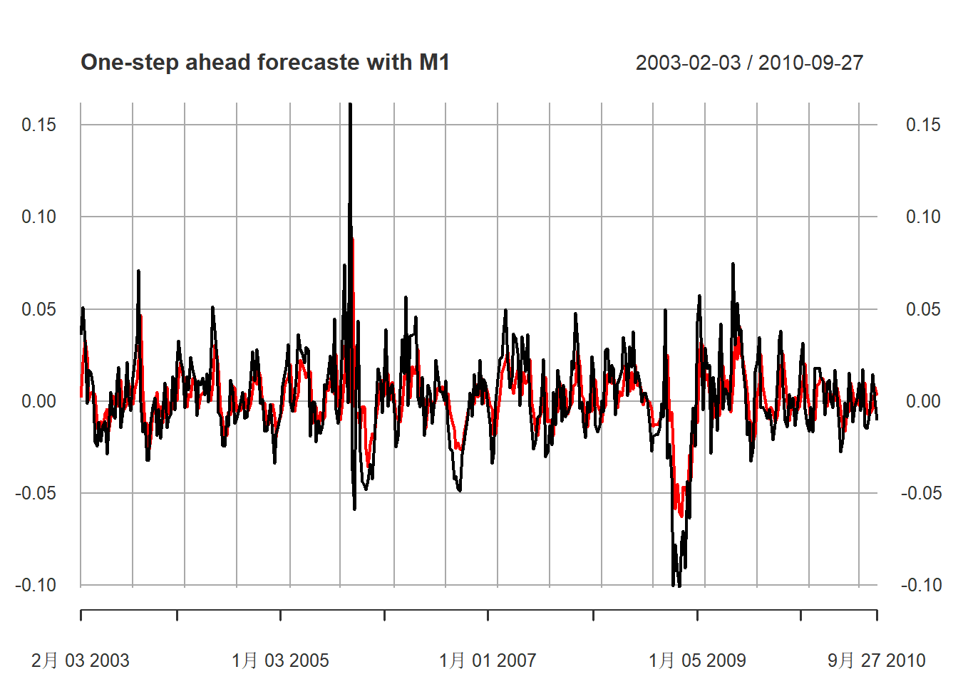
图15.21: 汽油价格对数增长率用M1模型做一步预测
M2模型的预报图,黑色为真实值, 红色为预报值:
xts.p2 <- xts(cbind(dpgs1[nmin:nmax], fcst[nmin:nmax,2]),
              index(xts.pgs)[-(1:2)][nmin:nmax])
plot(xts.p2, type="l",
     main="One-step ahead forecaste with M2",
     major.ticks="years", minor.ticks=NULL,
     col=c("black", "red"))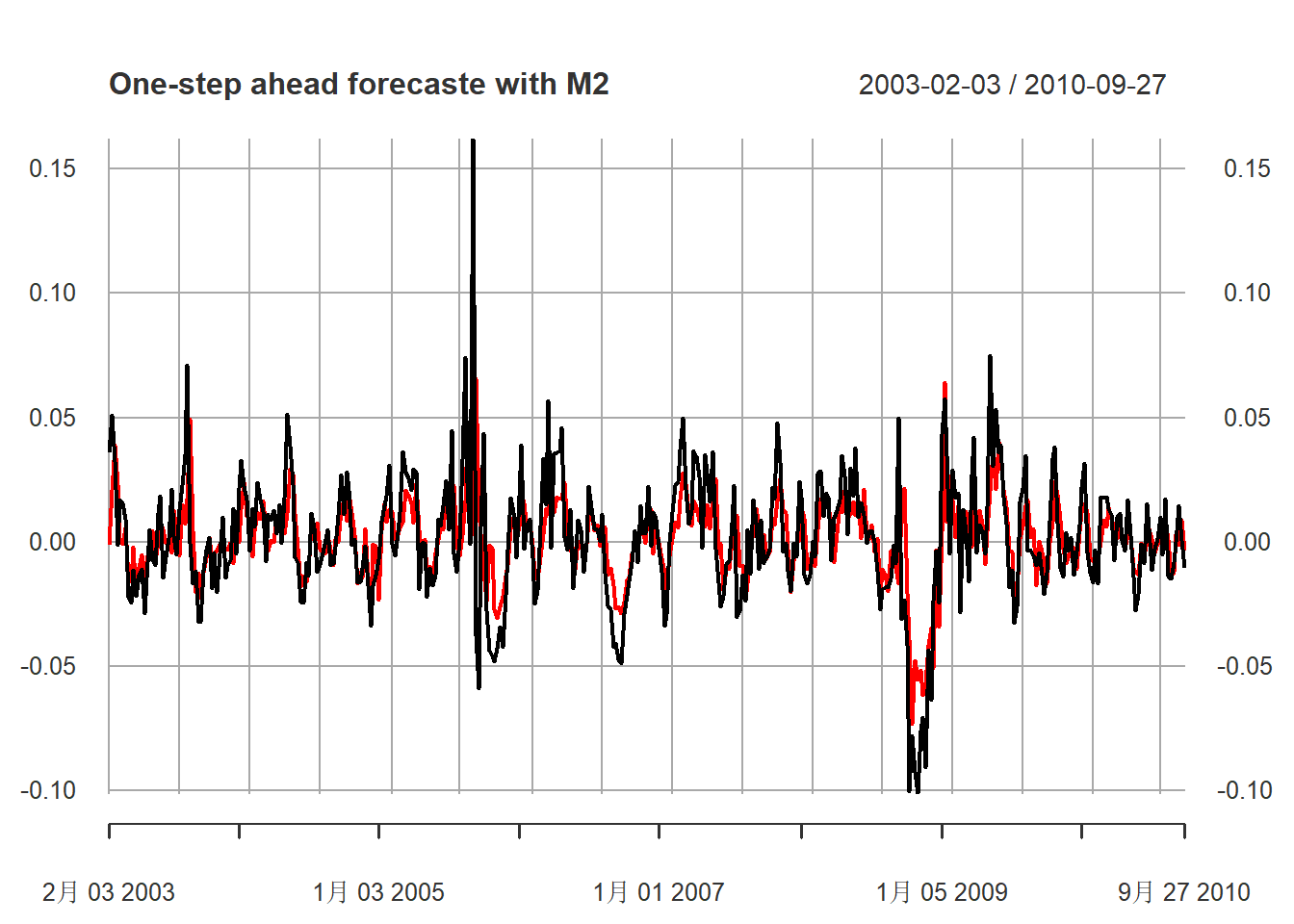
图15.22: 汽油价格对数增长率用M2模型做一步预测
如果从图形看, 可以看出超前一步预测还是有一定效果的。