15 线性时间序列案例学习—美国月失业率

失业率是每个国家、地区经济运行的重要指标。 2011年，美国的季节调整后的月度失业率在9%左右。

本章对美国月失业率数据进行建模和预测， 使用不带解释变量和带解释变量的两种方法， 解释变量是周首次申请失业救济金人数信息。

数据来自Department of Labor, US Beareau of Labor Statistics。 数据经过了季节调整。 失业率为百分数(单位是%)， 是16周岁及以上的失业人口比例。 每周首次申请失业救济金人数是每周新的申请失业保险的人数。 失业率月度数据，从1948年1月到2010年9月， 每月的第一天报告。 周首次申请失业救济金人数是周数据， 有效数据从1967-01-07到2010-08-28， 每周六报告。

本案例的目的是：

1. 演示混合频率的时间序列的分析方法（这里是月频与周频）；
2. 强调季节调整过的数据的建模有潜在的模型设置错误；
3. 说明基于先验经验的试错法在模型设置中有帮助。

15.1 单变量时间序列模型

失业率数据从1948年1月到2010年9月，共753个观测值。

读入数据：

da <- read_table("m-unrate.txt", col_types = cols(.default = col_double()))
xts.unrate <- xts(
  da[["rate"]], with(da, make_date(Year, mon, dd)))
tclass(xts.unrate) <- "yearmon"
ts.unrate <- ts(da[["rate"]], start=c(1948,1), frequency = 12)
ts.dur <- diff(ts.unrate)

作时间序列图：

plot(
  xts.unrate, ylim=c(0, 12),
  main="US Monthly Unemployment Rate",
  major.ticks="years", minor.ticks=NULL, 
  grid.ticks.on="years",
  col="red"
)

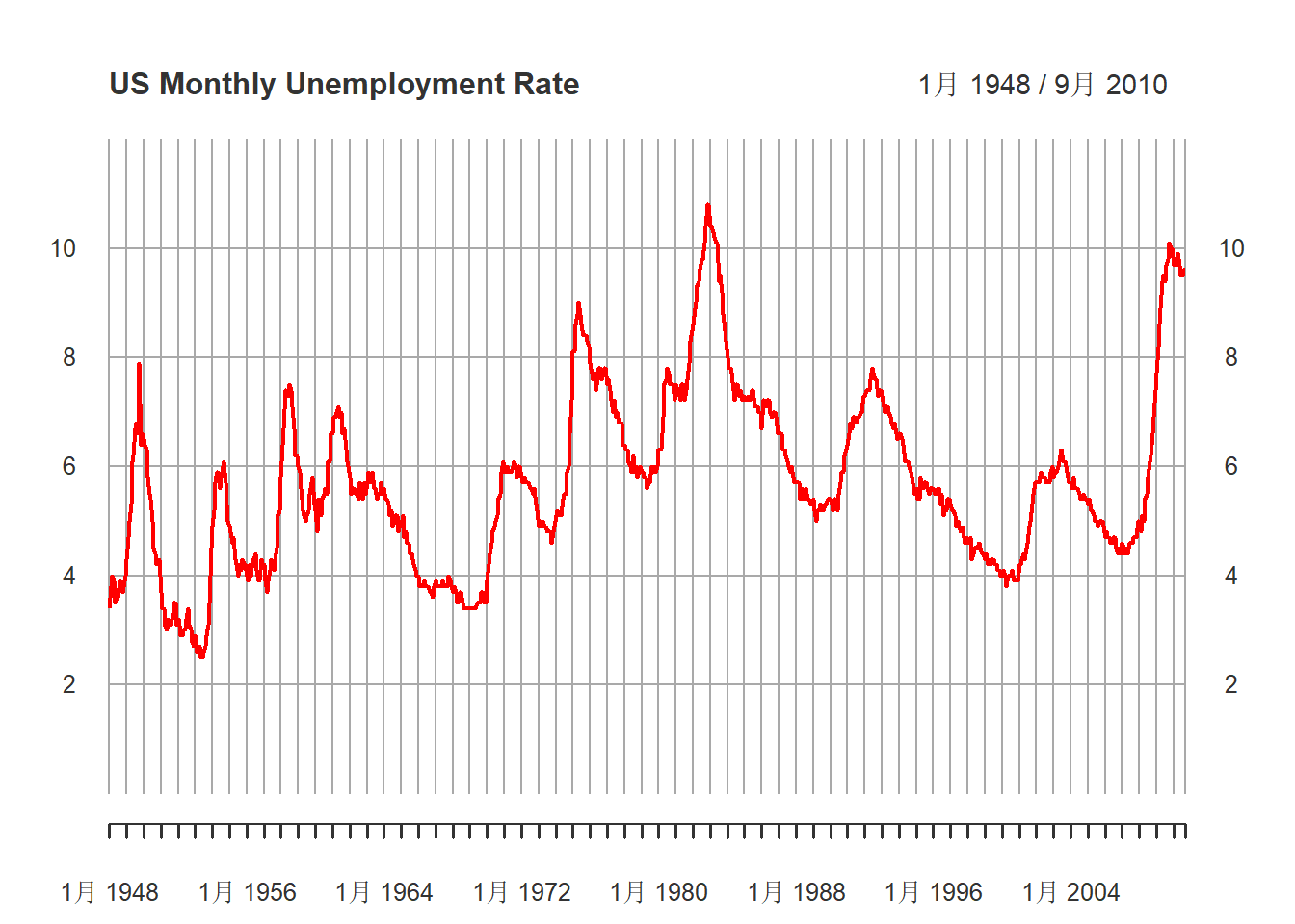
图15.1: 美国月度失业率（经季节调整后）

分段作时间序列图：

plot(
  xts.unrate["1948/1968"], ylim=c(0, 12),
  main="US Monthly Unemployment Rate",
  major.ticks="years", minor.ticks=NULL, 
  grid.ticks.on="years",
  col="red"
)

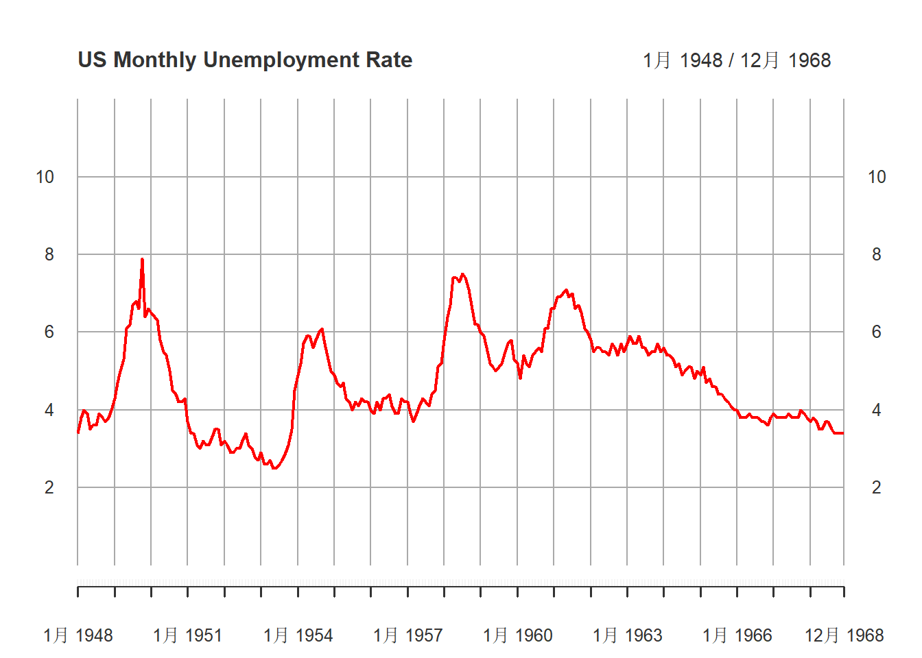
图15.2: 美国月度失业率（经季节调整后）1948-1968

plot(
  xts.unrate["1968/1988"], ylim=c(0, 12),
  main="US Monthly Unemployment Rate",
  major.ticks="years", minor.ticks=NULL, 
  grid.ticks.on="years",
  col="red"
)

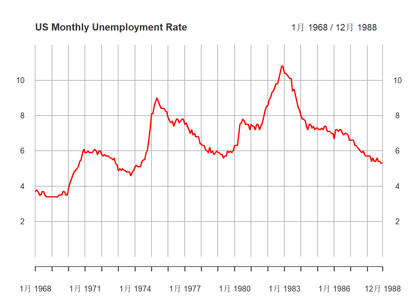
图15.3: 美国月度失业率（经季节调整后）1968-1988

plot(
  xts.unrate["1988/"], ylim=c(0, 12),
  main="US Monthly Unemployment Rate",
  major.ticks="years", minor.ticks=NULL, 
  grid.ticks.on="years",
  col="red"
)

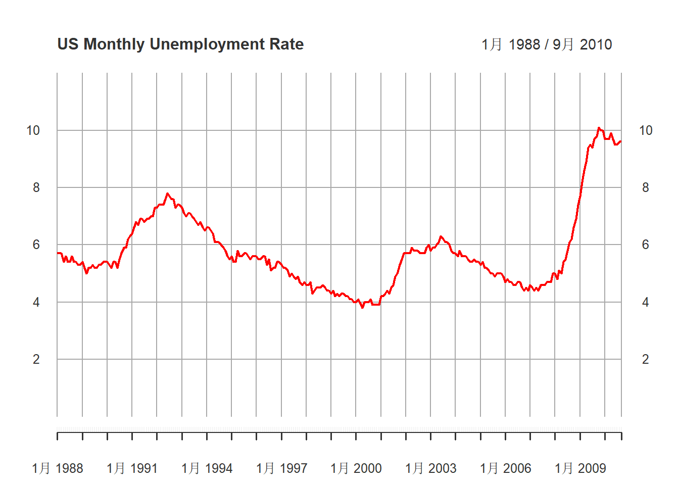
图15.4: 美国月度失业率（经季节调整后）1988-2010

观察失业率的月度时间序列图发现：

1. 失业率有周期性变化，但周期不固定；
2. 失业率水平在数据的时间范围内可能有增长趋势；
3. 失业率上升快，下降慢。这预示着失业率序列不服从线性时间序列。 这里先不使用非线性时间序列。

记\(x_t\)为月度失业率序列， 作其ACF图：

acf(ts.unrate, lag.max=36, main="")

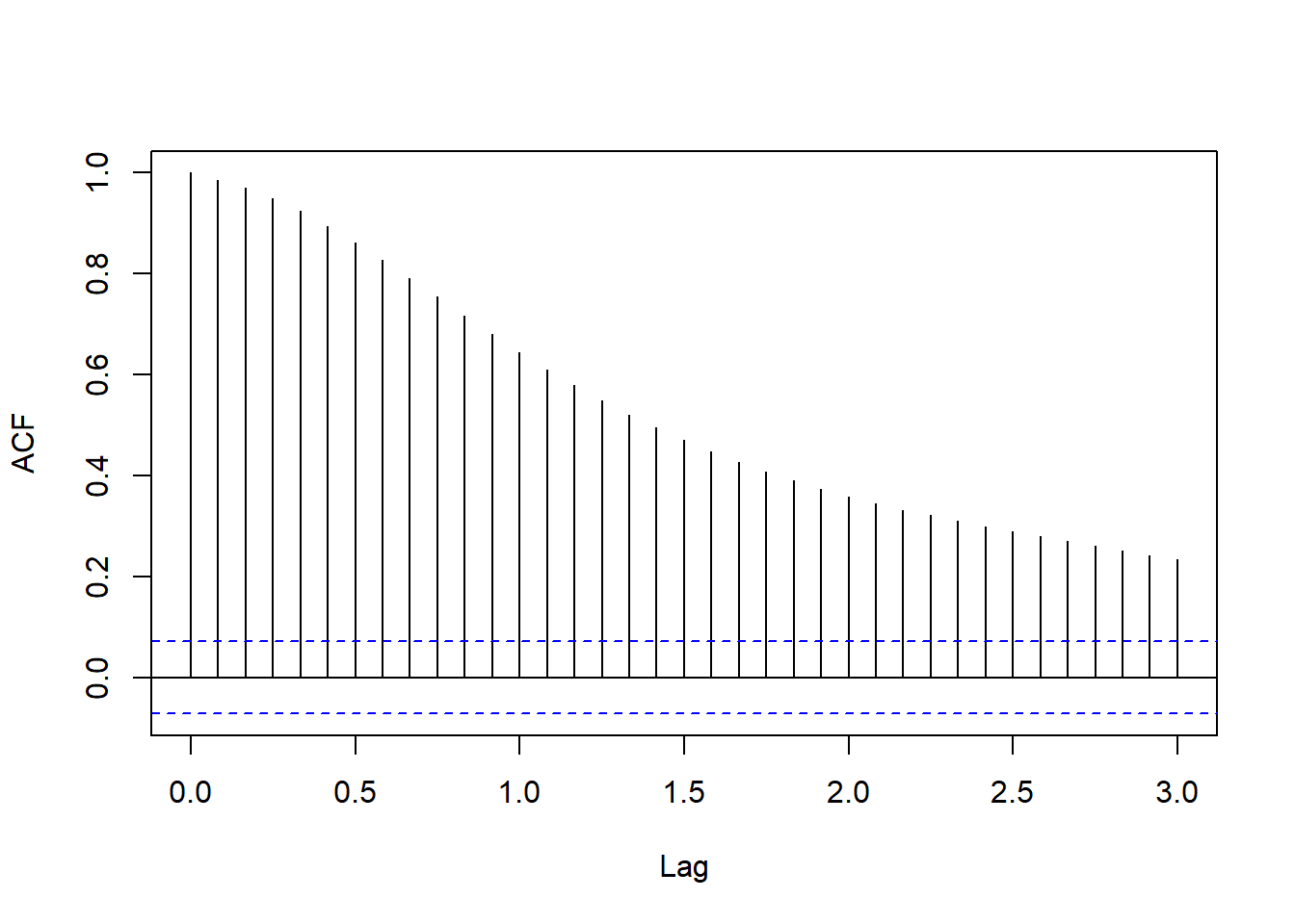
图15.5: 美国月度失业率的ACF

这像是单位根非平稳。 计算其差分序列，作ACF图：

forecast::Acf(ts.dur, lag.max=36, main="")

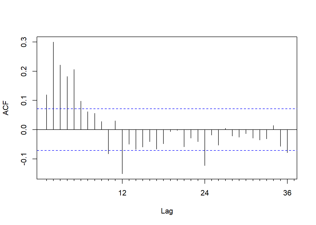
图15.6: 美国月度失业率差分的ACF

这不太像是低阶的MA， 在周期12的倍数有较高相关， 怀疑是季节调整的残余周期性。

差分序列的PACF:

pacf(ts.dur, lag.max=36, main="")

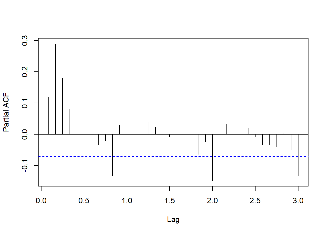
图15.7: 美国月度失业率差分的PACF

这也不像是低阶的AR， 而且在周期12的整倍数的偏自相关也超出。

对差分序列用AIC定阶建立AR模型：

ar(ts.dur, method="mle")

## 
## Call:
## ar(x = ts.dur, method = "mle")
## 
## Coefficients:
##       1        2        3        4        5        6        7        8  
##  0.0114   0.2208   0.1536   0.1030   0.1319   0.0007  -0.0333   0.0047  
##       9       10       11       12  
## -0.0056  -0.1032   0.0302  -0.1174  
## 
## Order selected 12  sigma^2 estimated as  0.03838

作单位根检验：

fUnitRoots::adfTest(ts.unrate, lags=12, type="ct")

## 
## Title:
##  Augmented Dickey-Fuller Test
## 
## Test Results:
##   PARAMETER:
##     Lag Order: 12
##   STATISTIC:
##     Dickey-Fuller: -2.8364
##   P VALUE:
##     0.2243 
## 
## Description:
##  Wed Mar 23 07:35:56 2022 by user: Lenovo

检验结果不显著，说明有单位根。

总结以上所见：

• 失业率序列很可能是单位根过程；
• 尽管已经进行了季节调整， 差分序列的ACF和PACF在滞后为12倍数的地方还是较高， 说明序列仍残余12个月周期的影响， 可能还需要在模型中考虑增加季节项；
• 差分序列的ACF和PACF在滞后为12倍数处数值约0.15， 但是衰减很慢， 这有些像是长记忆过程， 当ARMA方程两边有相近特征根时可表现出类似长记忆性质；
• 除了季节性外，差分序列的ACF和PACF在5阶或6阶显著， PACF指数震荡衰减；
• 可尝试\(p=1\)和\(q=5\)。 取\(q=5\)是考虑到PACF的震荡衰减以及ACF在前5阶较高。 取\(p=1\)是因为ACF也是指数衰减而不是快速截尾。

因此尝试如下的带有季节性的 ARIMA\((1,1,5)(1,0,1)_{12}\)模型：

resm <- arima(
  ts.unrate, order=c(1,1,5),
  seasonal=list(order=c(1,0,1), period=12)
)
resm

## 
## Call:
## arima(x = ts.unrate, order = c(1, 1, 5), seasonal = list(order = c(1, 0, 1), 
##     period = 12))
## 
## Coefficients:
##          ar1      ma1     ma2     ma3     ma4     ma5    sar1     sma1
##       0.7301  -0.7468  0.2194  0.0073  0.0383  0.0831  0.5978  -0.8469
## s.e.  0.0686   0.0776  0.0462  0.0501  0.0467  0.0431  0.0672   0.0477
## 
## sigma^2 estimated as 0.03643:  log likelihood = 176.43,  aic = -334.87

删去不显著的MA3和MA4系数：

mod1 <- arima(
  ts.unrate, order=c(1,1,5),
  seasonal=list(order=c(1,0,1), period=12),
  fixed=c(NA, NA, NA, 0, 0, NA, NA, NA)
)
mod1

## 
## Call:
## arima(x = ts.unrate, order = c(1, 1, 5), seasonal = list(order = c(1, 0, 1), 
##     period = 12), fixed = c(NA, NA, NA, 0, 0, NA, NA, NA))
## 
## Coefficients:
##          ar1      ma1     ma2  ma3  ma4     ma5    sar1     sma1
##       0.7536  -0.7744  0.2351    0    0  0.0990  0.6051  -0.8525
## s.e.  0.0569   0.0650  0.0365    0    0  0.0386  0.0654   0.0457
## 
## sigma^2 estimated as 0.03649:  log likelihood = 175.75,  aic = -337.5

作模型残差检验：

tsdiag(mod1, gof=36)

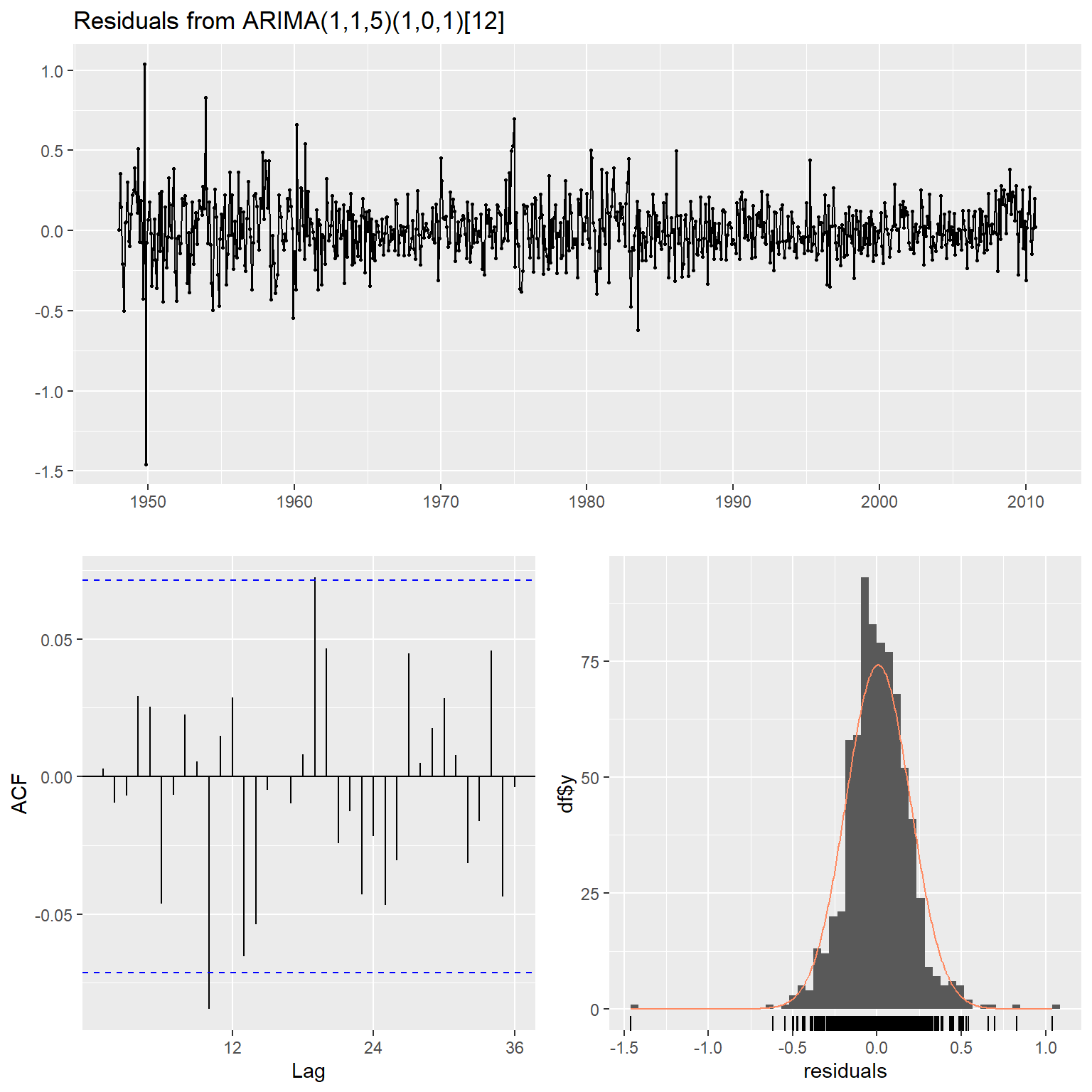
图15.8: 失业率ARIMA模型的残差检验

结果表明模型充分。 模型可以写成

\[\begin{align} & (1 - 0.61 B^{12}) (1 - 0.75B) (1 - B) x_t \\ =& (1 - 0.85 B^{12}) (1 - 0.77 B + 0.24 B^2 + 0.099 B^5) \varepsilon_t, \\ & \quad \text{Var}(\varepsilon_t) = 0.0365, \quad \text{AIC}=-337.5 \tag{15.1} \end{align}\]

15.2 一个替代模型

因为考虑到需要有季节项， 所以可以先建立一个仅有差分和季节项的模型， 对残差分析再考虑增加其他AR或者MA成分。

resm2 <- arima(
  ts.unrate, order=c(0,1,0),
  seasonal=list(order=c(1,0,1), period=12)
)
resm2

## 
## Call:
## arima(x = ts.unrate, order = c(0, 1, 0), seasonal = list(order = c(1, 0, 1), 
##     period = 12))
## 
## Coefficients:
##         sar1     sma1
##       0.6195  -0.8670
## s.e.  0.0658   0.0468
## 
## sigma^2 estimated as 0.04267:  log likelihood = 116.9,  aic = -227.8

拟合的模型为 \[ (1 - 0.62 B^{12}) x_t = (1 - 0.87 B^{12}) b_t, \ \sigma_b^2 = 0.04267 \] 其中\(b_t\)表示残差序列。 考察\(b_t\)的ACF和PACF：

forecast::Acf(resm2$residuals, lag.max=36, main="")

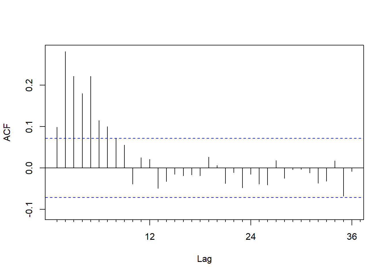
图15.9: 单变量仅季节项的残差ACF

残差ACF明显在前6阶不为零。

pacf(resm2$residuals, lag.max=36, main="")

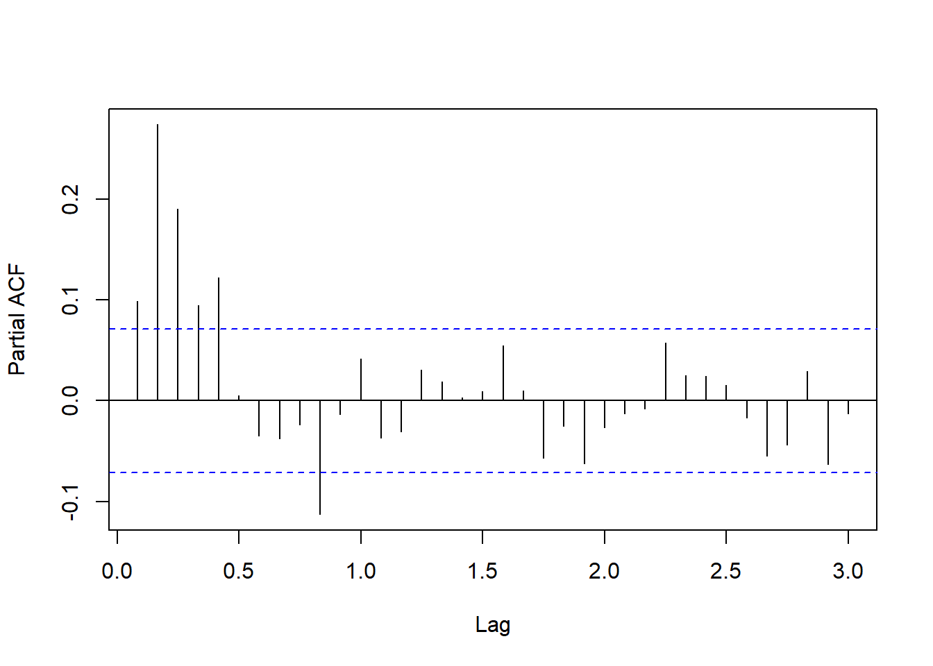
图15.10: 单变量仅季节项的残差PACF

PACF呈现指数速度震荡衰减。 所以，怀疑残差仍有5阶或6阶以上的MA，

从PACF观察， 尝试建立一个AR(5)：

resm3 <- arima(
  ts.unrate, order=c(5,1,0),
  seasonal=list(order=c(1,0,1), period=12)
)
resm3

## 
## Call:
## arima(x = ts.unrate, order = c(5, 1, 0), seasonal = list(order = c(1, 0, 1), 
##     period = 12))
## 
## Coefficients:
##           ar1     ar2     ar3     ar4     ar5    sar1     sma1
##       -0.0124  0.2101  0.1682  0.1024  0.1207  0.5624  -0.8233
## s.e.   0.0365  0.0366  0.0366  0.0370  0.0366  0.0723   0.0526
## 
## sigma^2 estimated as 0.03663:  log likelihood = 174.57,  aic = -333.13

删去不显著的ar1系数：

fixed <- rep(NA_real_, 7); fixed[1] <- 0
mod2 <- arima(
  ts.unrate, order=c(5,1,0),
  seasonal=list(order=c(1,0,1), period=12),
  fixed=fixed
)

## Warning in arima(ts.unrate, order = c(5, 1, 0), seasonal = list(order = c(1, :
## some AR parameters were fixed: setting transform.pars = FALSE

mod2

## 
## Call:
## arima(x = ts.unrate, order = c(5, 1, 0), seasonal = list(order = c(1, 0, 1), 
##     period = 12), fixed = fixed)
## 
## Coefficients:
##       ar1     ar2     ar3     ar4     ar5    sar1     sma1
##         0  0.2104  0.1652  0.0996  0.1194  0.5643  -0.8240
## s.e.    0  0.0366  0.0355  0.0362  0.0364  0.0724   0.0528
## 
## sigma^2 estimated as 0.03664:  log likelihood = 174.51,  aic = -335.02

其AIC的值为-335，比mod1的AIC=-337略差一些。

模型可以写成：

\[\begin{align} & (1 - 0.56 B^{12})(1 - 0.21B^2 - 0.17 B^3 - 0.10 B^4 - 0.12 B^5) (1 - B) x_t \\ =& (1 - 0.82 B^{12}) \varepsilon_t, \quad \sigma_{\varepsilon}^2 = 0.03664, \quad \text{AIC}=-335 \tag{15.2} \end{align}\]

模型检验：

tsdiag(mod2, gof=36)

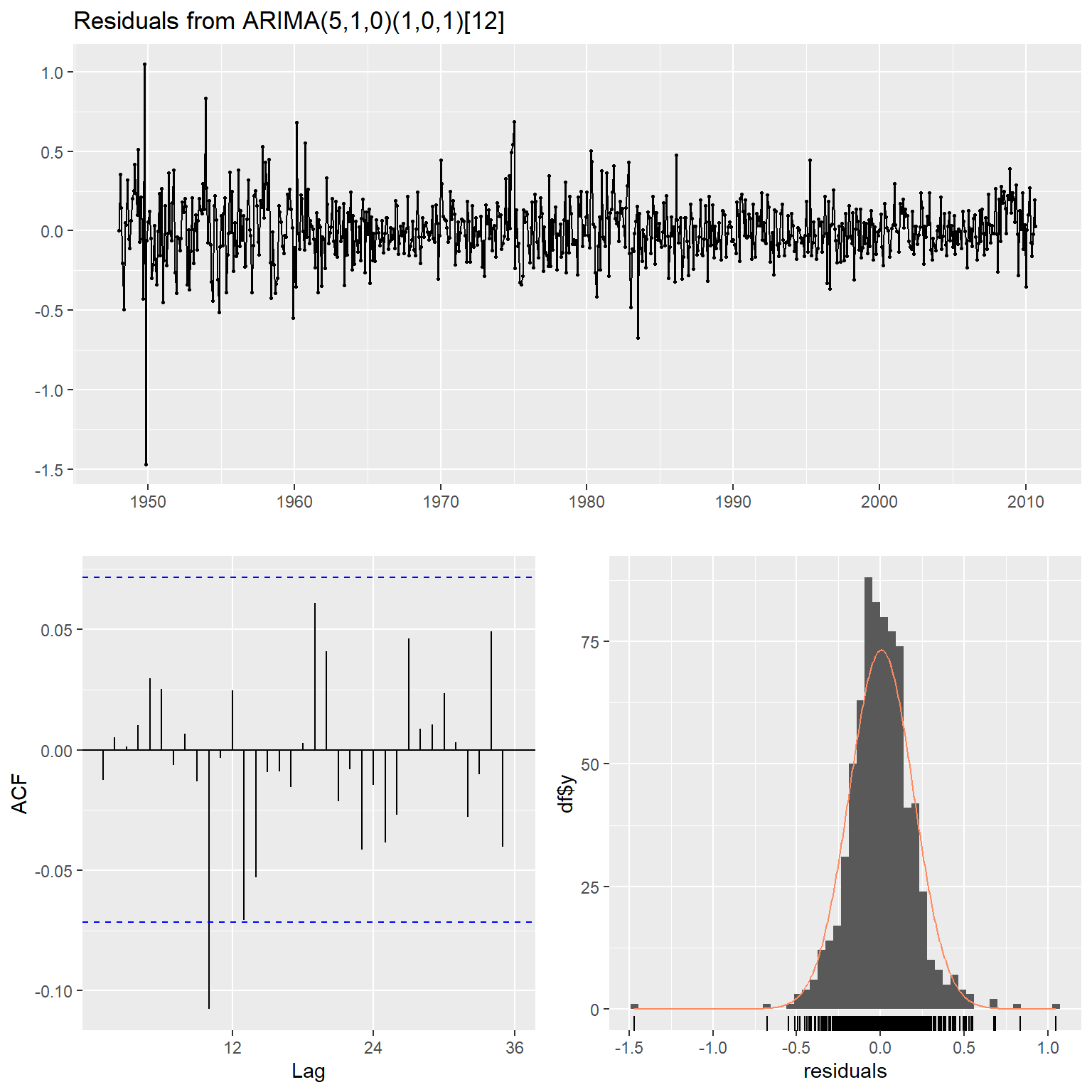
图15.11: 单变量候选模型检验

此模型也可以接受。

15.3 模型比较

比较(15.1)的mod1和(15.2)的mod2。

• 从残差诊断来看，两个模型都很合适。
• 从AIC比较，mod1为\(-337\)，mod2为\(-335\)，mod1略占优。

下面进行样本外比较。 保留样本的最后53个观测值， 共有753个观测值， 初始使用前700个建模， 逐步地作超前一步预报。

使用mod1作超前一步预报的函数为：

pred1 <- function(y=ts.unrate, n.pred=73){
  T <- length(y)
  ypred <- rep(NA_real_, T)
  for(h in (T-n.pred):(T-1)){
    mod <- arima(
      y[1:h], order=c(1,1,5),
      seasonal=list(order=c(1,0,1), period=12),
      fixed=c(NA, NA, NA, 0, 0, NA, NA, NA)
    )
    ypred[h+1] <- predict(mod, n.ahead=1, se.fit=FALSE)
  }
  
  ypred
}

使用mod2作超前一步预报的函数为：

pred2 <- function(y=ts.unrate, n.pred=73){
  T <- length(y)
  ypred <- rep(NA_real_, T)
  fixed <- rep(NA_real_, 7); fixed[1] <- 0
  for(h in (T-n.pred):(T-1)){
    mod <- arima(
      y[1:h], order=c(5,1,0),
      seasonal=list(order=c(1,0,1), period=12),
      fixed=fixed, transform.pars=FALSE
    )
    ypred[h+1] <- predict(mod, n.ahead=1, se.fit=FALSE)
  }
  
  ypred
}

对一种方法的预测计算预测根均方误差(RMFSE)和平均绝对预测误差(MAFE)的函数：

pred.err <- function(y, n.pred=length(ypred), ypred){
  T <- length(y)
  i1 <- T - n.pred + 1
  RMFSE <- sqrt( mean((y[i1:T] - ypred[i1:T])^2) )
  MAFE <- mean(abs(y[i1:T] - ypred[i1:T]))
  
  c(RMFSE=RMFSE, MAFE=MAFE)
}

样本外预测比较：

err1 <- pred.err(y=ts.unrate, n.pred=73, 
                 ypred=pred1(ts.unrate, n.pred=73))
err2 <- pred.err(y=ts.unrate, n.pred=73, 
                 ypred=pred2(ts.unrate, n.pred=73))
err.tab1 <- data.frame(
  Model=c("mod1", "mod2"),
  RMFSE=c(err1[["RMFSE"]], err2[["RMFSE"]]),
  MAFE=c(err1[["MAFE"]], err2[["MAFE"]])
)
knitr::kable(err.tab1, digits=4)

Model	RMFSE	MAFE
mod1	0.1503	0.1182
mod2	0.1514	0.1185

两个模型的样本外预测效果也不相上下， mod1略占优。 事实上， 如果不考虑季节因素， 将AR改写成MA表示， 两个模型十分接近。

15.4 使用首次申请失业救济金人数

这一节用周首次申请失业救济金人数作为解释变量来预测失业率。 因为申请人数数据是从1967年1月开始才有， 所以尽管失业率数据从1948年1月开始就有， 我们要使用共同的数据存在的期间。

因为每个月的1号报告失业率， 为了预报失业率只能使用前一个月的申请人数数据。 实际使用的失业率数据跨度为1967年2月到2010年9月， 周首次申请失业救济金人数数据跨度为1967年1月到2010年8月。 用到的失业率的有效数据点数为524个。

周频数据与月频数据如何匹配？ 一种办法是将\(x_t\)对应的第\(t-1\)月的所有周的申请人数加起来得到一个解释变量\(c_{t-1}\)， 就频率相同了。 另一种办法是将第\(t-1\)个月的前4周的申请人数 \(w_{1,t-1}, w_{2,t-1}, w_{3,t-1}, w_{4,t-1}\)都作为解释变量， 如果有第5周也不用， \(c_{t-1}\)不一定等于这四个变量的和。 为避免数值计算量纲差距太大， 申请人数原来以千人为单位，改为以百万人为单位。

da2 <- read_table("m-unrateic.txt", 
                   col_types = cols(.default = col_double()))
da2[,5:9] <- da2[,5:9]/1000
xts.unic <- xts(
  da2[,-(1:3)], with(da2, make_date(year, mon, dd)))
tclass(xts.unic) <- "yearmon"
unrate <- da2[["rate"]]
head(da2)

## # A tibble: 6 x 9
##    year   mon    dd  rate  w1m1  w2m1  w3m1  w4m1  icm1
##   <dbl> <dbl> <dbl> <dbl> <dbl> <dbl> <dbl> <dbl> <dbl>
## 1  1967     2     1   3.8 0.208 0.207 0.217 0.204 0.836
## 2  1967     3     1   3.8 0.216 0.229 0.229 0.242 0.916
## 3  1967     4     1   3.8 0.31  0.241 0.245 0.247 1.04 
## 4  1967     5     1   3.8 0.259 0.257 0.299 0.245 1.32 
## 5  1967     6     1   3.9 0.254 0.231 0.23  0.228 0.943
## 6  1967     7     1   3.8 0.248 0.238 0.224 0.218 0.928

两个序列的图形：

plot(xts.unic[,c("rate", "icm1")],
     multi.panel=TRUE, yaxis.same=FALSE,
     main="月失业率与上个月申请失业救济金人数（单位：百万人）",
     major.ticks="years", minor.ticks=NULL, 
     grid.ticks.on="years",
     col=c("red", "green"))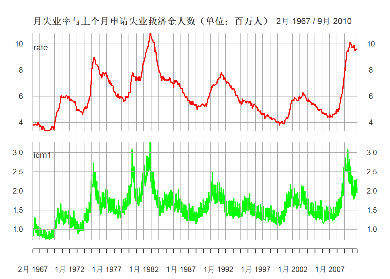

图15.12: 月失业率与上个月申请失业救济金人数（单位：百万人）

失业率对上个月申请人数的散点图：

plot(da2[["icm1"]], da2[["rate"]], type="p",
     pch=16, col="gray",
     xlab="上个月申请失业救济金人数（单位：百万人）",
     ylab="月失业率")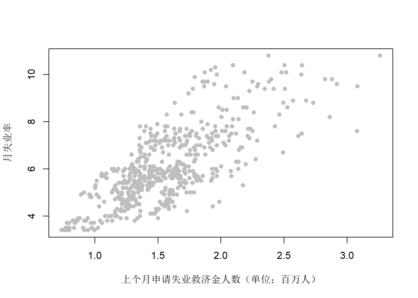

图15.13: 月失业率对上个月申请失业救济金人数

两者存在一定的线性相关性。相关系数：

cor(da2[["icm1"]], da2[["rate"]])

## [1] 0.7570642

15.4.1 使用前一月申请人数总和

图15.13给出了从1967年2月到2010年9月的月失业率\(x_t\)的时序图， 以及对应的前一个月的首次申请失业救济金人数的\(c_{t-1}\)序列的时序图。 可以看出两者呈现一种共同的运动。

先拟合一个简单的一元线性回归模型：

lm1 <- lm(rate ~ icm1, data=da2)
summary(lm1)

## 
## Call:
## lm(formula = rate ~ icm1, data = da2)
## 
## Residuals:
##     Min      1Q  Median      3Q     Max 
## -2.8638 -0.7008 -0.1299  0.7366  3.1746 
## 
## Coefficients:
##             Estimate Std. Error t value Pr(>|t|)    
## (Intercept)   1.5202     0.1785   8.518   <2e-16 ***
## icm1          2.9047     0.1097  26.475   <2e-16 ***
## ---
## Signif. codes:  0 '***' 0.001 '**' 0.01 '*' 0.05 '.' 0.1 ' ' 1
## 
## Residual standard error: 1.051 on 522 degrees of freedom
## Multiple R-squared:  0.5731, Adjusted R-squared:  0.5723 
## F-statistic: 700.9 on 1 and 522 DF,  p-value: < 2.2e-16

结果的回归复相关系数平方为0.57， 说明有一定预报能力。 模型为 \[ x_t = 1.52 + 2.905 c_{t-1} + n_t \] 其中\(n_t\)为误差项。

但是，这个回归有两个问题：

• 残差很可能有序列自相关， 使得回归的检验是不可用的， 估计也不是最有效的；
• 如果回归因变量和自变量存在单位根非平稳， 结果可能是虚假的。

回归残差的ACF:

lm1 <- lm(rate ~ icm1, data=da2)
acf(lm1$residuals, lag.max=36, main="")

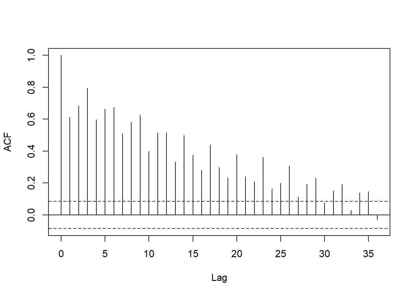
图15.14: 以月申请人数为解释变量的回归残差的ACF

残差的ACF衰减缓慢， 可能由于原始序列有单位根。

回归残差的PACF:

lm1 <- lm(rate ~ icm1, data=da2)
pacf(lm1$residuals, lag.max=36, main="")

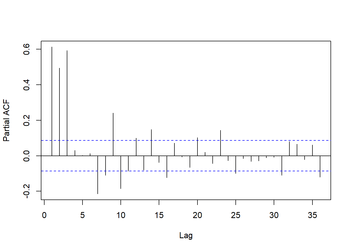
图15.15: 以月申请人数为解释变量的回归残差的PACF

前3个PACF很较高，后面也有多处超出界限。 从回归残差的ACF和PACF来看不一定能用ARMA模型建模。

为克服模型设定上的困难， 我们应用试错法和一些先验知识。

1. 由于是月度数据， 模型可能需要季节项。
2. 失业率呈现出一定的非固定的周期波动， 来源于商业周期， 这表明失业率模型的一些特征根是复根， 因此AR的阶在2以上；
3. 回归残差的ACF都是正的， 可考虑MA阶为整数，试选取\(q=3\)。

暂定失业率带有月申请人数解释变量的模型为： \[\begin{align} &(1 - \phi_1 B - \phi_2 B^2)(1 - \Phi B^{12})(x_t - \beta_0 - \beta_1 c_{t-1}) \\ =& (1 + \theta_1 B + \theta_2 B^2 + \theta_3 B^3) (1 + \Theta B^{12}) a_t \end{align}\]

resm4 <- arima(
  da2[["rate"]], xreg=da2[["icm1"]], 
  order=c(2,0,3),
  seasonal=list(order=c(1,0,1), period=12)
); resm4

## 
## Call:
## arima(x = da2[["rate"]], order = c(2, 0, 3), seasonal = list(order = c(1, 0, 
##     1), period = 12), xreg = da2[["icm1"]])
## 
## Coefficients:
##          ar1      ar2      ma1     ma2     ma3    sar1     sma1  intercept
##       1.8997  -0.9021  -0.8932  0.1458  0.0555  0.6501  -0.8520     6.0373
## s.e.  0.0332   0.0331   0.0543  0.0565  0.0466  0.0824   0.0586     0.3706
##       da2[["icm1"]]
##              0.0772
## s.e.         0.0212
## 
## sigma^2 estimated as 0.02419:  log likelihood = 227.7,  aic = -435.39

因为数据不同，这里的AIC不与前面的单变量模型比较。 结果表明ma3系数不显著，所以MA改为\(q=2\)建模：

mod3 <- arima(
  da2[["rate"]], xreg=da2[["icm1"]], 
  order=c(2,0,2),
  seasonal=list(order=c(1,0,1), period=12)
); mod3

## 
## Call:
## arima(x = da2[["rate"]], order = c(2, 0, 2), seasonal = list(order = c(1, 0, 
##     1), period = 12), xreg = da2[["icm1"]])
## 
## Coefficients:
##          ar1      ar2      ma1     ma2    sar1     sma1  intercept
##       1.9123  -0.9145  -0.9100  0.1860  0.6465  -0.8483     6.1111
## s.e.  0.0283   0.0282   0.0527  0.0479  0.0823   0.0591     0.3748
##       da2[["icm1"]]
##              0.0782
## s.e.         0.0213
## 
## sigma^2 estimated as 0.02426:  log likelihood = 226.97,  aic = -435.93

各个系数都显著。 模型的残差诊断：

tsdiag(mod3, gof=36)

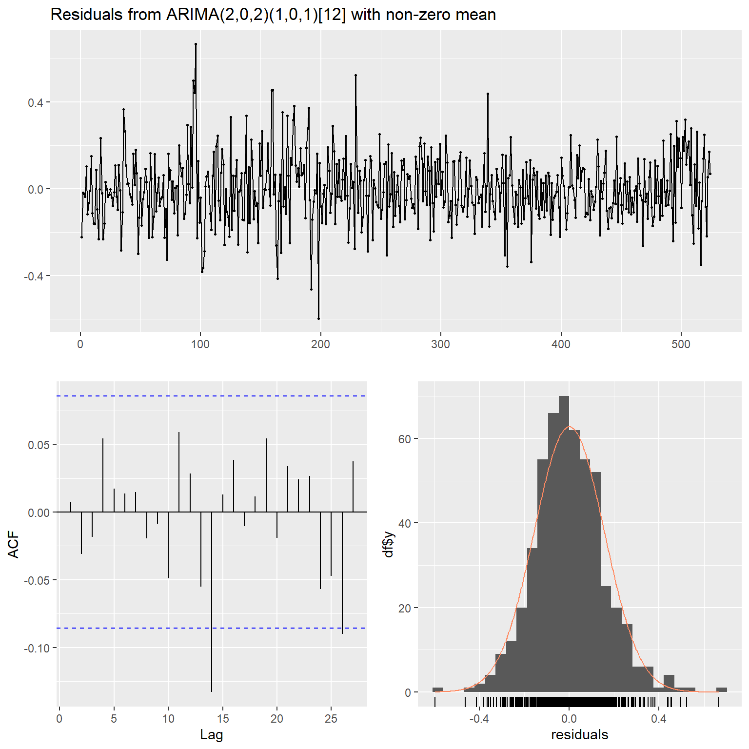
图15.16: 用月申请人数为解释变量的ARIMA模型的诊断

除了残差有较多异常值以外， 残差呈现出白噪声性质。

模型mod3可以写成：

\[\begin{align} & (1 - 1.91 B + 0.91 B^2) (1 - 0.65 B^{12}) (x_t - 6.11 - 0.0782 c_{t-1}) \\ =& (1 - 0.91 B + 0.18 B^2) (1 - 0.84 B^{12}) a_t, \ \text{Var}(a_t)=0.02426, \ \text{AIC}=-435.93 \tag{15.3} \end{align}\]

模型中季节项的两个系数比较接近， 这往往可以产生部分长记忆的现象。

模型中AR部分除了有一个对应于周期12的特征根以外， 其它的特征根和对应的周期为：

polyroot(c(1, -coef(mod3)[1:2]))

## [1] 1.045522+0.019388i 1.045522-0.019388i

2*pi/Arg(polyroot(c(1, -coef(mod3)[1:2]))[1])/12

## [1] 28.23933

模型代表的周期为28个月。

15.4.2 使用前一月各周申请人数

这里使用前一个月的前四周的申请人数都作为自变量。 下图为失业率与前一个月的前两周的申请人数的数据， 三个序列走势是相近的：

plot(xts.unic[,c("rate", "w1m1", "w2m1")],
     multi.panel=TRUE, yaxis.same=FALSE,
     main="月失业率与上个月前两周申请失业救济金人数（单位：百万人）",
     major.ticks="years", minor.ticks=NULL, 
     grid.ticks.on="years",
     col=c("red", "green", "cyan"))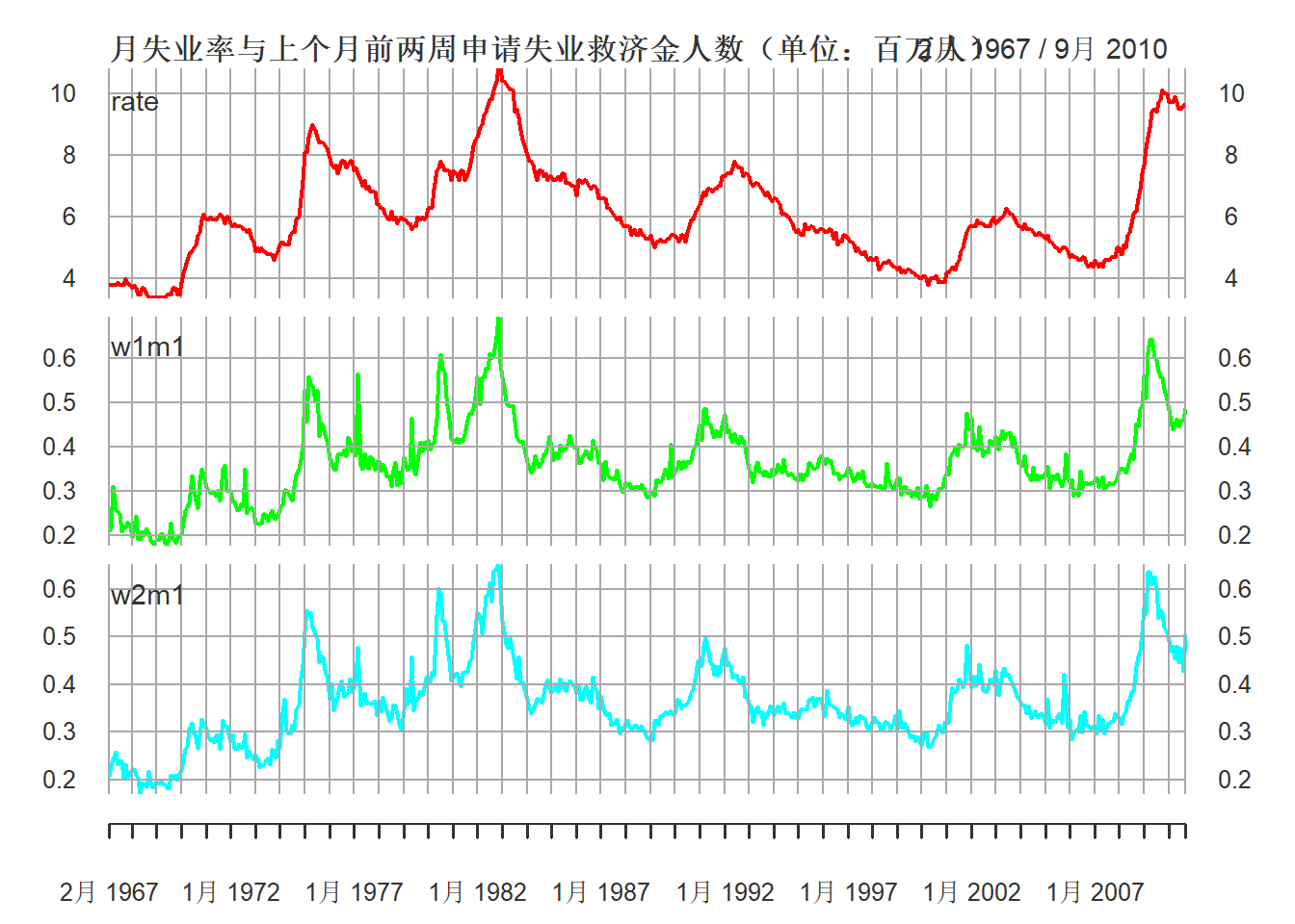

图15.17: 月失业率与上个月前两周申请失业救济金人数（单位：百万人）

用四个解释变量作多元线性回归：

lm2 <- lm(rate ~ w1m1 + w2m1 + w3m1 + w4m1, data=da2)
summary(lm2)

## 
## Call:
## lm(formula = rate ~ w1m1 + w2m1 + w3m1 + w4m1, data = da2)
## 
## Residuals:
##      Min       1Q   Median       3Q      Max 
## -2.40629 -0.67602 -0.06686  0.62419  2.55888 
## 
## Coefficients:
##             Estimate Std. Error t value Pr(>|t|)    
## (Intercept)   0.5160     0.1651   3.125 0.001877 ** 
## w1m1          6.5221     2.1145   3.084 0.002148 ** 
## w2m1          9.6711     2.8630   3.378 0.000785 ***
## w3m1         -2.4455     2.7980  -0.874 0.382506    
## w4m1          1.6626     2.0624   0.806 0.420528    
## ---
## Signif. codes:  0 '***' 0.001 '**' 0.01 '*' 0.05 '.' 0.1 ' ' 1
## 
## Residual standard error: 0.8841 on 519 degrees of freedom
## Multiple R-squared:  0.6998, Adjusted R-squared:  0.6975 
## F-statistic: 302.5 on 4 and 519 DF,  p-value: < 2.2e-16

复相关系数平方为0.70， 高于仅使用总数作为解释变量时的0.57。 当然， 线性回归每增加一个解释变量其复相关系数平方都会增加， 有过度拟合危险。 这个回归的可能问题与用总数作为解释变量的情形类似， 另外， 模型中后第三、四周的解释变量不显著。 这并不表明第三、四周的申请人数对下个月失业率没有预报能力， 而是其预报能力可以被第一、二周的数据代替。 比如， 仅使用第三、四周建模：

lm2b <- lm(rate ~ w3m1 + w4m1, data=da2)
summary(lm2b)

## 
## Call:
## lm(formula = rate ~ w3m1 + w4m1, data = da2)
## 
## Residuals:
##      Min       1Q   Median       3Q      Max 
## -2.62420 -0.69034 -0.07828  0.63761  2.89772 
## 
## Coefficients:
##             Estimate Std. Error t value Pr(>|t|)    
## (Intercept)   0.6694     0.1707   3.920   0.0001 ***
## w3m1         10.2363     2.1342   4.796 2.11e-06 ***
## w4m1          4.7578     2.1012   2.264   0.0240 *  
## ---
## Signif. codes:  0 '***' 0.001 '**' 0.01 '*' 0.05 '.' 0.1 ' ' 1
## 
## Residual standard error: 0.9226 on 521 degrees of freedom
## Multiple R-squared:  0.6718, Adjusted R-squared:  0.6706 
## F-statistic: 533.3 on 2 and 521 DF,  p-value: < 2.2e-16

结果仍是显著的。

下面仅使用第一、二周的申请人数预报下个月的失业率：

lm3 <- lm(rate ~ w1m1 + w2m1, data=da2)
summary(lm3)

## 
## Call:
## lm(formula = rate ~ w1m1 + w2m1, data = da2)
## 
## Residuals:
##      Min       1Q   Median       3Q      Max 
## -2.40653 -0.66933 -0.05949  0.63075  2.56954 
## 
## Coefficients:
##             Estimate Std. Error t value Pr(>|t|)    
## (Intercept)   0.5127     0.1647   3.113  0.00195 ** 
## w1m1          6.4594     2.0709   3.119  0.00191 ** 
## w2m1          8.9609     2.0872   4.293  2.1e-05 ***
## ---
## Signif. codes:  0 '***' 0.001 '**' 0.01 '*' 0.05 '.' 0.1 ' ' 1
## 
## Residual standard error: 0.8832 on 521 degrees of freedom
## Multiple R-squared:  0.6993, Adjusted R-squared:  0.6981 
## F-statistic: 605.8 on 2 and 521 DF,  p-value: < 2.2e-16

复相关系数平方仍为0.70， 相比使用四个解释变量的模型基本没有下降。

仅使用前两周的数据预报还有一个额外的好处， 就是给出预报的时间提前了， 可以在前一个月15号的时候就预报下个月的失业率， 如果使用总数则需要在月底才能预报下个月1号报告的失业率。

考察模型的残差ACF：

acf(lm3$residuals, lag.max=36, main="")

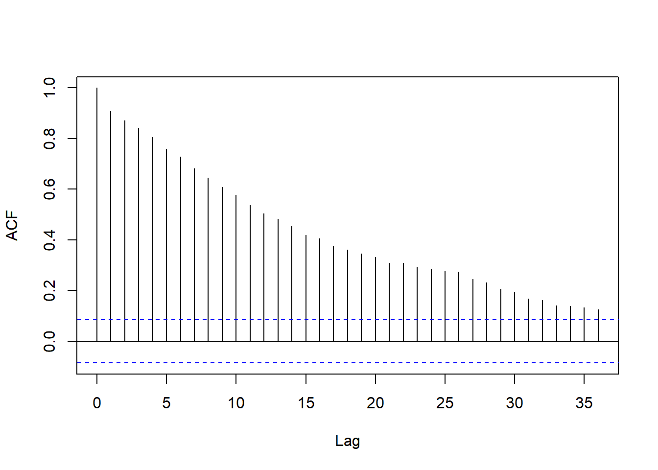
图15.18: 使用两周申请人数作为解释变量的回归残差ACF

回归残差ACF衰减缓慢， 怀疑有单位根残余。 相关系数都为正数。

pacf(lm3$residuals, lag.max=36, main="")

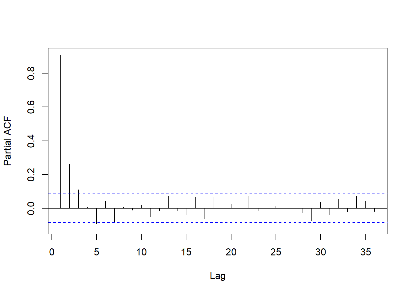
图15.19: 使用两周申请人数作为解释变量的回归残差PACF

这个PACF比较符合截尾特征， 取\(p=3\)可能合适。 使用与mod3类似的设定：

mod4 <- arima(
  da2[["rate"]], xreg=as.matrix(da2[,c("w1m1", "w2m1")]), 
  order=c(2,0,2),
  seasonal=list(order=c(1,0,1), period=12)
); mod4

## 
## Call:
## arima(x = da2[["rate"]], order = c(2, 0, 2), seasonal = list(order = c(1, 0, 
##     1), period = 12), xreg = as.matrix(da2[, c("w1m1", "w2m1")]))
## 
## Coefficients:
##          ar1      ar2      ma1     ma2    sar1     sma1  intercept    w1m1
##       1.9172  -0.9197  -0.9958  0.2532  0.6111  -0.7915     5.6555  0.4265
## s.e.  0.0269   0.0268   0.0563  0.0507  0.1119   0.0883     0.3912  0.2721
##         w2m1
##       0.9693
## s.e.  0.3206
## 
## sigma^2 estimated as 0.024:  log likelihood = 230.29,  aic = -440.59

模型AIC为\(-440.59\)，小于mod3的\(-435.93\)。 样本内比较mod4优于mod3。

mod4模型残差诊断：

tsdiag(mod4, gof=36)

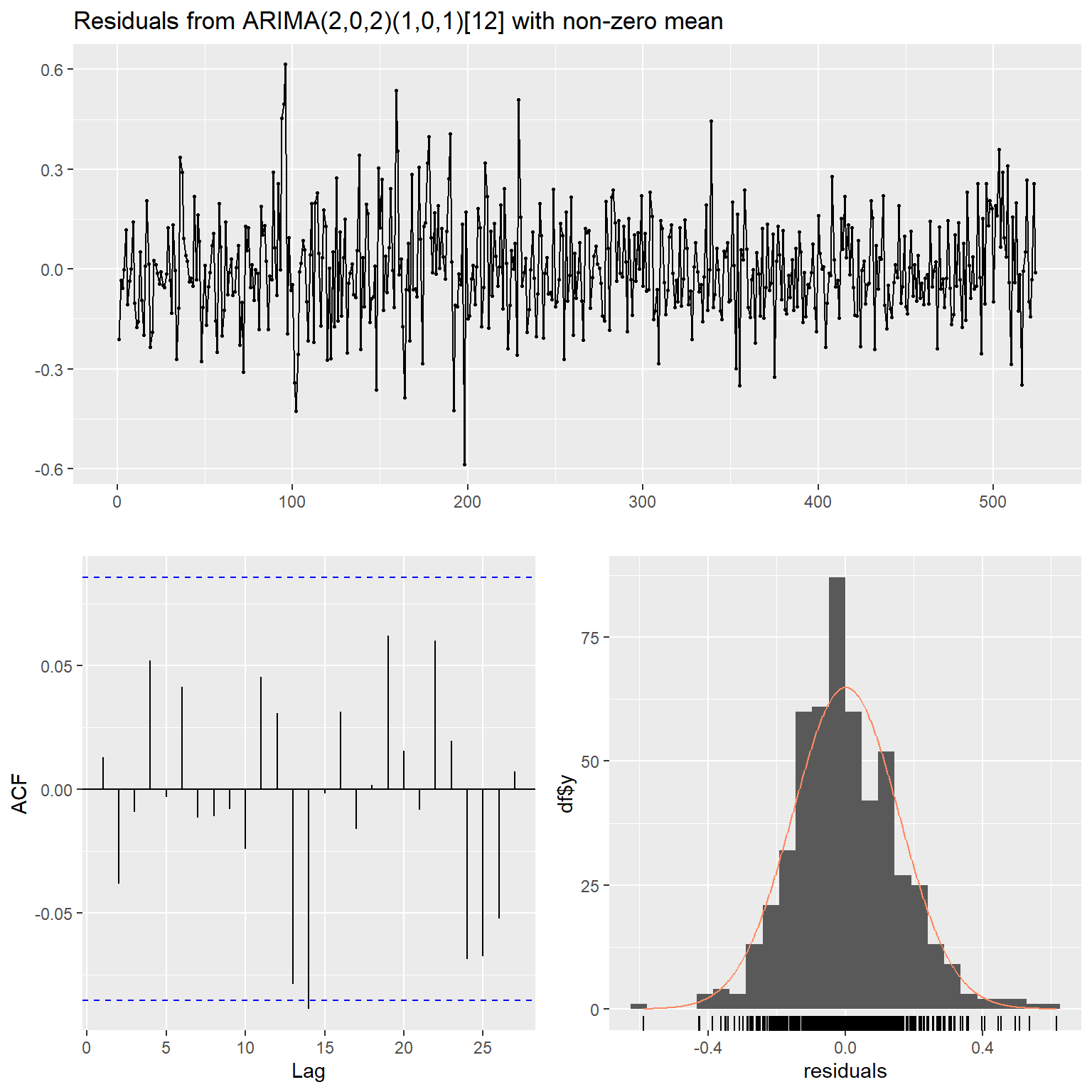
图15.20: 使用前两周申请人数为解释变量的ARIMA模型的残差诊断

残差诊断可以接受。

模型mod4公式为：

\[\begin{align} &(1 - 1.92 B + 0.92 B^2) (1 - 0.61 B^{12}) (x_t - 5.66 - 0.4265 w_{1,t-1} - 0.9693 w_{2,t-1}) \\ =& (1 - 1.00 B + 0.25 B^2) (1 - 0.79 B^{12}) a_t, \ \text{Var}(a_t)=0.024, \ \text{AIC}=-4440.59 \tag{15.4} \end{align}\]

仔细比较mod3和mod4， 可以发现回归残差的ARMA模型的系数基本相同。

15.5 模型再比较

前面的利用上个月首次申请失业救济金人数为解释变量的模型应该更准确地预测月失业率。 为了比较， 再建立一个不利用解释变量的单变量时间序列模型， 时间期间取相同的可比的1967年2月到2010年9月。

mod5 <- arima(
  da2[["rate"]],
  order=c(1,1,2),
  seasonal=list(order=c(1,0,1), period=12)
); mod5

## 
## Call:
## arima(x = da2[["rate"]], order = c(1, 1, 2), seasonal = list(order = c(1, 0, 
##     1), period = 12))
## 
## Coefficients:
##          ar1      ma1     ma2    sar1     sma1
##       0.9007  -0.8684  0.1700  0.6250  -0.8303
## s.e.  0.0310   0.0532  0.0467  0.0838   0.0615
## 
## sigma^2 estimated as 0.0252:  log likelihood = 219.08,  aic = -426.17

模型mod5的残差诊断：

tsdiag(mod5, gof=36)

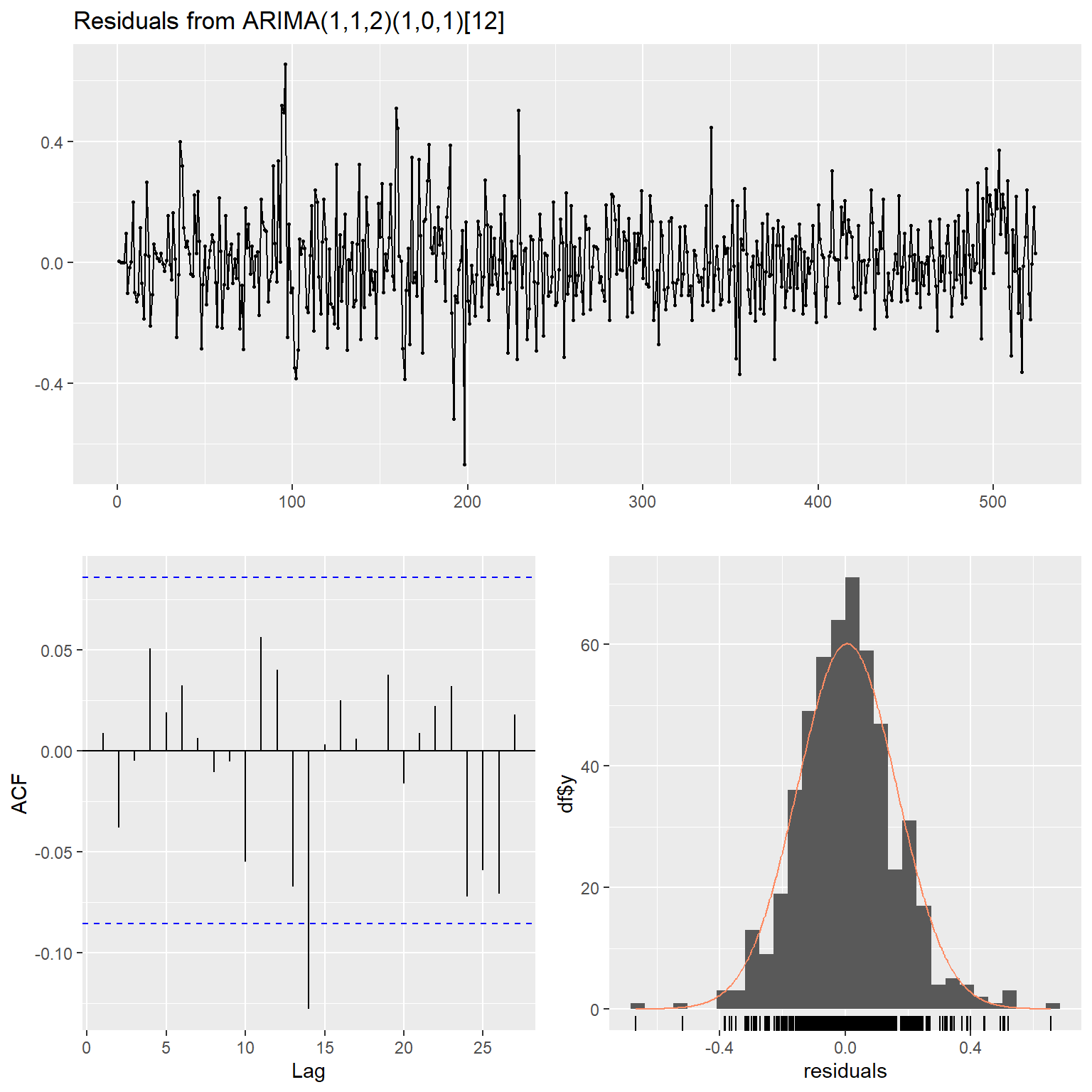
图15.21: 时间区间缩短的一元时间序列的残差诊断

残差诊断表明模型mod5可接受。 模型公式： \[\begin{align} (1 - 0.90 B) (1 - B) (1 - 0.63B^{12}) x_t =& (1 - 0.87 B + 0.17 B^2)(1 - 0.83 B^{12}) a_t \\ \text{Var}(a_t)=& 0.0252, \ \text{AIC} = -426.7 \tag{15.5} \end{align}\]

用AIC作样本内比较：

err.tab2 <- data.frame(
  "模型"=c("使用月申请人数", "使用两周申请人数", "不使用解释变量"),
  AIC=c(-435.93, -440.59, -426.17))
knitr::kable(err.tab2)

模型	AIC
使用月申请人数	-435.93
使用两周申请人数	-440.59
不使用解释变量	-426.17

用AIC作样本内比较， 使用两周申请人数的模型mod4最优， 不使用解释变量的模型mod5最差。

下面进行样本外比较。保留最后53个月数据用于预测比较。

使用mod3作超前一步预报的函数为：

pred3 <- function(da=da2, n.pred=53){
  T <- nrow(da)
  ypred <- rep(NA_real_, T)
  for(h in (T-n.pred):(T-1)){
    mod <- arima(
      da[["rate"]][1:h], xreg=da[["icm1"]][1:h], 
      order=c(2,0,2),
      seasonal=list(order=c(1,0,1), period=12)
    )
    ypred[h+1] <- predict(mod, n.ahead=1, se.fit=FALSE,
                          newxreg=cbind(da[["icm1"]][h+1]))
  }
  
  ypred
}

使用mod4作超前一步预报的函数为：

pred4 <- function(da=da2, n.pred=53){
  T <- nrow(da)
  ypred <- rep(NA_real_, T)
  for(h in (T-n.pred):(T-1)){
    mod <- arima(
      da[["rate"]][1:h], xreg=as.matrix(da2[1:h,c("w1m1", "w2m1")]), 
      order=c(2,0,2),
      seasonal=list(order=c(1,0,1), period=12)
    )
    ypred[h+1] <- predict(mod, n.ahead=1, se.fit=FALSE,
                          newxreg=cbind(da[["w1m1"]][h+1], da[["w2m1"]][h+1]))
  }
  
  ypred
}

使用mod5作超前一步预报的函数为：

pred5 <- function(da=da2, n.pred=53){
  T <- nrow(da)
  ypred <- rep(NA_real_, T)
  for(h in (T-n.pred):(T-1)){
    mod <- arima(
      da[["rate"]][1:h],
      order=c(1,1,2),
      seasonal=list(order=c(1,0,1), period=12)
    )
    ypred[h+1] <- predict(mod, n.ahead=1, se.fit=FALSE)
  }
  
  ypred
}

对一种方法的预测计算预测根均方误差(RMFSE)和平均绝对预测误差(MAFE)的函数：

样本外比较的计算：

pred.tab3 <- data.frame(
  "模型"=c("使用月申请人数", "使用两周申请人数", "不使用解释变量"),
  AIC=c(-435.93, -440.59, -426.17),
  RMFSE=rep(0.0, 3),
  MAFE=rep(0.0, 3)
)
funcs <- list(pred3, pred4, pred5)
for(i in 1:3){
  predf <- funcs[[i]]
  ypred <- predf(da=da2, n.pred=53)
  err <- pred.err(y=da2[["rate"]], n.pred=53, ypred=ypred)
  pred.tab3[i, "RMFSE"] <- err["RMFSE"]
  pred.tab3[i, "MAFE"] <- err["MAFE"]
}

## Warning in arima(da[["rate"]][1:h], xreg = da[["icm1"]][1:h], order = c(2, :
## possible convergence problem: optim gave code = 1

## Warning in arima(da[["rate"]][1:h], xreg = da[["icm1"]][1:h], order = c(2, :
## possible convergence problem: optim gave code = 1

## Warning in arima(da[["rate"]][1:h], xreg = da[["icm1"]][1:h], order = c(2, :
## possible convergence problem: optim gave code = 1

## Warning in arima(da[["rate"]][1:h], xreg = da[["icm1"]][1:h], order = c(2, :
## possible convergence problem: optim gave code = 1

## Warning in arima(da[["rate"]][1:h], xreg = da[["icm1"]][1:h], order = c(2, :
## possible convergence problem: optim gave code = 1

## Warning in arima(da[["rate"]][1:h], xreg = da[["icm1"]][1:h], order = c(2, :
## possible convergence problem: optim gave code = 1

## Warning in arima(da[["rate"]][1:h], xreg = da[["icm1"]][1:h], order = c(2, :
## possible convergence problem: optim gave code = 1

## Warning in arima(da[["rate"]][1:h], xreg = da[["icm1"]][1:h], order = c(2, :
## possible convergence problem: optim gave code = 1

## Warning in arima(da[["rate"]][1:h], xreg = da[["icm1"]][1:h], order = c(2, :
## possible convergence problem: optim gave code = 1

## Warning in arima(da[["rate"]][1:h], xreg = da[["icm1"]][1:h], order = c(2, :
## possible convergence problem: optim gave code = 1

## Warning in arima(da[["rate"]][1:h], xreg = da[["icm1"]][1:h], order = c(2, :
## possible convergence problem: optim gave code = 1

## Warning in arima(da[["rate"]][1:h], xreg = da[["icm1"]][1:h], order = c(2, :
## possible convergence problem: optim gave code = 1

## Warning in arima(da[["rate"]][1:h], xreg = as.matrix(da2[1:h, c("w1m1", :
## possible convergence problem: optim gave code = 1

## Warning in arima(da[["rate"]][1:h], xreg = as.matrix(da2[1:h, c("w1m1", :
## possible convergence problem: optim gave code = 1

## Warning in arima(da[["rate"]][1:h], xreg = as.matrix(da2[1:h, c("w1m1", :
## possible convergence problem: optim gave code = 1

## Warning in arima(da[["rate"]][1:h], xreg = as.matrix(da2[1:h, c("w1m1", :
## possible convergence problem: optim gave code = 1

## Warning in arima(da[["rate"]][1:h], xreg = as.matrix(da2[1:h, c("w1m1", :
## possible convergence problem: optim gave code = 1

## Warning in arima(da[["rate"]][1:h], xreg = as.matrix(da2[1:h, c("w1m1", :
## possible convergence problem: optim gave code = 1

## Warning in arima(da[["rate"]][1:h], xreg = as.matrix(da2[1:h, c("w1m1", :
## possible convergence problem: optim gave code = 1

## Warning in arima(da[["rate"]][1:h], xreg = as.matrix(da2[1:h, c("w1m1", :
## possible convergence problem: optim gave code = 1

## Warning in arima(da[["rate"]][1:h], xreg = as.matrix(da2[1:h, c("w1m1", :
## possible convergence problem: optim gave code = 1

knitr::kable(pred.tab3, digits=4)

模型	AIC	RMFSE	MAFE
使用月申请人数	-435.93	0.1706	0.1454
使用两周申请人数	-440.59	0.1683	0.1372
不使用解释变量	-426.17	0.1684	0.1370

计算过程中出现多次建模时参数估计的最优化程序不收敛。

样本外比较与样本内比较结果很不同， 样本内比较时， 使用解释变量的模型明显较优。 但是样本外比较时一元时间序列模型不差甚至于更优。 这可能和仅超前一步预报有关， 单位根模型在超前一步预报时基本上是用前一个数值作为超前一步预报的值， 因为月失业率数据变化较慢， 所以单位根模型也能得到较好的超前一步预测结果。

这个例子展示了样本内比较与样本外比较的差别。

三个模型有许多相似性：

第一，都有季节项，说明虽然序列都进行过季节调整， 但仍残余季节影响；

第二，使用解释变量的模型(15.3)、(15.4) 虽然没有单位根， 但是其特征根很接近于有单位根的情形：

abs(polyroot(c(1, -coef(mod3)[1:2])))

## [1] 1.045701 1.045701

abs(polyroot(c(1, -coef(mod4)[1:2])))

## [1] 1.042751 1.042751

这从一个侧面也解释了三个模型的超前一步预测效果相近的原因。