28 状态空间模型

上一章的局部水平模型是线性高斯状态空间模型的一个简单特例。本章给出状态空间模型，举例说明这种模型能够表示的其它模型，如ARIMA模型，结构时间序列模型，时变回归模型，有自相关误差的回归模型，随机波动率模型等，并给出滤波、平滑、预报公式和参数估计方法。

参考：

(Durbin and Koopman 2012)
(Tsay 2010)
(Beijers 2020)

28.1 状态空间模型的公式

28.1.1 线性高斯状态空间模型

状态空间模型有许多不同的表达形式，按照(Durbin and Koopman 2012)的公式，线性高斯模型为： \[\begin{align} \boldsymbol y_t =& Z_t \boldsymbol \alpha_t + \boldsymbol \varepsilon_t, \ \boldsymbol \varepsilon_t \sim \text{N}(0, H_t), \tag{28.1} \\ \boldsymbol \alpha_{t+1} =& T_t \boldsymbol \alpha_t + R_t \boldsymbol \eta_t, \ \boldsymbol \eta_t \sim \text{N}(0, Q_t), \tag{28.2} \end{align}\] 其中\(\boldsymbol y_t\)是\(t\)时刻的观测值，为\(p \times 1\)向量； \(\boldsymbol \alpha_t\)时\(t\)时刻系统的状态，是不可观测的\(m\times 1\)随机向量，第一个方程称为观测方程，第二个方程称为状态方程。 \(\{\boldsymbol \varepsilon_t\}\)和\(\{\boldsymbol \eta_t \}\)相互独立，都是独立同分布向量白噪声列， \(\boldsymbol \varepsilon_t\)为\(p\times 1\)随机向量， \(\boldsymbol \eta_t\)为\(r \times 1\)随机向量，\(r \leq m\)。设各矩阵\(Z_t, T_t, R_t, H_t, Q_t\)已知， \(Z_t\)和\(T_{t-1}\)允许依赖于\(\boldsymbol y_1, \dots, \boldsymbol y_{t-1}\)，初始状态\(\boldsymbol\alpha_1\)服从\(N(\boldsymbol a_1, P_1)\)，设\(\boldsymbol a_1, P_1\)已知， \(\boldsymbol\alpha_1\)与\(\{\boldsymbol \varepsilon_t\}\)和\(\{\boldsymbol \eta_t \}\)独立。当参数未知时，设\(\boldsymbol\psi\)为未知参数，矩阵\(Z_t, T_t, R_t, H_t, Q_t\)可以依赖于未知参数\(\boldsymbol\psi\)。

模型中的\(R_t\)常常是单位阵，\(r=m\)，有些教材的模型就没有\(R_t\)这一项。包含\(R_t\)的好处是， \(R_t\)常常是单位阵\(I_m\)的某些列组成的一个\(m \times r\)矩阵，称为选择矩阵，这允许某些状态分量对应的方程误差为0，同时\(\boldsymbol \eta_t\)的方差阵\(Q_t\)还可以是满秩的\(r \times r\)正定阵，如果没有\(R_t\)矩阵\(Q_t\)就可能不满秩。如果\(R_t\)是一般的\(m \times r\)矩阵，关于状态空间模型的大部分结论仍成立。

28.1.2 推广的状态空间模型

可以将线性高斯的状态空间模型，推广到状态方程仍为线性高斯形式，而观测方程的分布为非高斯分布，或者观测方程中观测变量与状态变量的关系非线性，更进一步可以推广到状态方程的关系也非线性，分布为非高斯分布。

较一般的非线性、非高斯状态空间模型形式为： \[\begin{aligned} \boldsymbol y_t \sim& f_t(\boldsymbol\alpha_t; \boldsymbol\beta), \\ \boldsymbol\alpha_{t+1} \sim& g_t(\boldsymbol\alpha_t; \boldsymbol\theta), \end{aligned}\] 其中\(f_t(\cdot)\), \(g(\cdot)\)是密度函数或概率质量函数， \(\boldsymbol\beta\)和\(\boldsymbol\theta\)是超参数。这样的模型一般需要用MCMC、序贯重要抽样等随机模拟方法进行滤波、平滑和估计。

28.1.3 MARSS包的模型

(Holmes, Scheuerell, and Ward 2021)中的状态空间模型与(Durbin and Koopman 2012)的模型形式相近，但更加灵活。有配套的扩展包MARSS， MARSS是多元自回归状态空间模型的缩写，实际上就是线性高斯状态空间模型。

基本的模型公式为： \[\begin{aligned} \boldsymbol x_t =&\ B \boldsymbol x_{t-1} + \boldsymbol u + \boldsymbol w_t, && \boldsymbol w_t \sim \text{N}(0, Q), \\ \boldsymbol y_t =&\ Z \boldsymbol x_t + \boldsymbol a + \boldsymbol v_t, && \boldsymbol v_t \sim \text{N}(0, R), \\ \boldsymbol x_0 \sim&\ \text{N}(\boldsymbol \pi, \Lambda) . \end{aligned} \tag{28.3} \] 这与(Durbin and Koopman 2012)的公式基本相同，只是记号不同，并且多出了\(\boldsymbol a\)和\(\boldsymbol u\)。矩阵\(B\), \(Z\), \(\boldsymbol u\), \(\boldsymbol a\)都允许时变。更复杂的模型还可以在两个方程中增加关于外生变量影响的部分。 MARSS扩展包的参数化方法和估计方法与其它状态空间模型扩展包有比较大的区别。

包含外生变量的回归部分并且各个矩阵允许时变的模型可以写成 \[\begin{aligned} \boldsymbol x_t =&\ B_t \boldsymbol x_{t-1} + \boldsymbol u_t + C_t \boldsymbol c_t + \boldsymbol w_t, && \boldsymbol w_t \sim \text{N}(0, Q_t), \\ \boldsymbol y_t =&\ Z_t \boldsymbol x_t + \boldsymbol a_t + D_t \boldsymbol d_t + \boldsymbol v_t, && \boldsymbol v_t \sim \text{N}(0, R_t), \\ \boldsymbol x_0 \sim&\ \text{N}(\boldsymbol \pi, \Lambda) . \end{aligned} \tag{28.4} \] 其中\(\boldsymbol c_t\)是系统方程中的\(p\)维外生变量数据，可以输入为一个\(p \times T\)矩阵； \(C_t\)是相应的回归载荷矩阵，可以包含未知量，如果是非时变的，只要输入为\(m \times p\)矩阵；如果是时变的，则需要输入为\(m \times p \times T\)的三维数组，用最后一个下标表示时间\(t\)。 \(\boldsymbol d_t\)则是观测方程中的\(q\)维外生变量数据， \(D_t\)是相应的载荷矩阵。

这样的MARSS模型不仅可以表示回归模型，也可以表示有内生状态变量\(\boldsymbol x_t\)的带有外生变量（回归自变量）的时间序列模型。

28.1.4 动态线性模型

(West and Harrison 1997)基于贝叶斯理论框架提出了高斯的动态线性模型，其结构和结果与线性高斯时间序列模型卡尔曼滤波基本相同。

用\(\boldsymbol \theta_t\)表示\(t\)时刻的状态， \(\boldsymbol y_t\)是\(t\)时刻的因变量， \(D_{t-1}\)表示\(t\)时刻之前的已知信息，则\(p(\boldsymbol \theta_t | D_{t-1})\)是\(t\)时刻的先验分布，相当于状态的一步预报分布， \(p(\boldsymbol \theta_t | D_t)\)是\(t\)的后验分布，相当于滤波分布，有 \[ p(\boldsymbol y_t, \boldsymbol \theta_t | D_{t-1}) = p(\boldsymbol y_t | \boldsymbol \theta_t, D_{t-1}) p(\boldsymbol \theta_t | D_{t-1}) . \] 可以从上述联合分布得到一步预报分布\(p(\boldsymbol y_t | D_{t-1})\)。

多元形式的高斯动态线性模型为： \[\begin{align} \boldsymbol Y_t | \boldsymbol \theta_t \sim&\ \text{N}[F_t^T \boldsymbol \theta_t, V_t], \tag{28.5} \\ \boldsymbol \theta_t | \boldsymbol \theta_{t-1} \sim&\ \text{N}[G_t \boldsymbol \theta_{t-1}, W_t] . \tag{28.6} \end{align}\] 或写成： \[\begin{aligned} \boldsymbol Y_t =&\ F_t^T \boldsymbol \theta_t + \boldsymbol \nu_t, && \boldsymbol \nu_t \sim \text{N}(0, V_t), \\ \boldsymbol \theta_t =&\ G_t \boldsymbol \theta_{t-1} + \boldsymbol \omega_t, && \boldsymbol \omega_t \sim \text{N}(0, W_t) , \\ &&& \boldsymbol \theta_0 \sim\ \text{N}(\boldsymbol m_0, C_0) . \end{aligned}\]

与(Durbin and Koopman 2012)的模型记号对比，上面的\(\boldsymbol \theta_t\)相当于\(\boldsymbol \alpha_t\)， \(F_t^T\)相当于\(Z_t\)， \(V_t\)相当于\(H_t\)， \(G_t\)相当于\(T_{t-1}\)， \(W_t\)相当于\(R_{t-1}=I\)时的\(Q_{t-1}\)。 ((28.5))-((28.6))中的分布也可以依赖于\(D_{t-1}\)。模型中的四个矩阵\((F_t, G_t, V_t, W_t)\)为非随机的超参数。

对于常见的线性时间序列模型， \((F_t, G_t, V_t, W_t)\)一般不依赖于\(t\)。

例28.1 (局部水平模型) 局部水平模型用DLM表示，是单个参数的一元时间序列模型。公式为： \[\begin{aligned} Y_t =&\ F_t \mu_t + \nu_t, && \nu_t \sim \text{N}(0, V_t), \\ \mu_t =&\ \lambda \mu_{t-1} + \omega_t, && \omega_t \sim \text{N}(0, W_t), \\ &&& (\mu_0 | D_0) \sim \text{N}(m_0, C_0) . \end{aligned}\] 其中\(F_t\), \(\lambda\)已知， \(V_t\)和\(W_t\)可以是未知的。当\(F_t=1\), \(\lambda=1\)则为一般的局部水平模型，在(West and Harrison 1997)中称为一阶多项式模型： \[\begin{aligned} Y_t =&\ \mu_t + \nu_t, && \nu_t \sim \text{N}(0, V_t), \\ \mu_t =&\ \mu_{t-1} + \omega_t, && \omega_t \sim \text{N}(0, W_t), \\ &&& (\mu_0 | D_0) \sim \text{N}(m_0, C_0) . \end{aligned}\] 其中\(W_t\)应该接近于0， \(\mu_t\)在短期内变化很小。

例28.2 (时变系数回归模型) 对时间序列使用线性回归，当不同时期的关系有缓慢变化时不能自动调整关系，可以推广为系数缓慢变化的模型。模型公式： \[\begin{aligned} y_t =&\ \alpha_t + \beta_t X_t + \nu_t, && \nu_t \sim \text{N}(0, V), \\ \alpha_t =&\ \alpha_{t-1} + \xi_t, && \xi_t \sim \text{N}(0, W^{(\alpha)}), \\ \beta_t =&\ \beta_{t-1} + \eta_t, && \eta_t \sim \text{N}(0, W^{(\beta)}) . \end{aligned}\] 其中\(W^{(\alpha)}\)和\(W^{(\beta)}\)都很接近于0。

28.2 有关R扩展包

R软件中有许多扩展包支持进行状态空间模型建模。

statespacer：支持线性高斯状态时间序列建模。
KFAS：支持线性高斯状态时间序列建模，也支持指数分布族的非高斯情况。
dlm：使用(West and Harrison 1997)的模型，动态线性模型。支持线性高斯时间序列模型，可使用最大似然估计，支持时变模型。
dynr：支持带有机制切换的离散时间或者连续时间的模型建模。
dse: 线性高斯的ARMA、VAR和状态空间模型，所用的方法不太符合R的使用习惯。
bssm: 非线性、非高斯状态空间模型的贝叶斯推断。
MARSS: 多元自回归状态空间模型。参数可以时变，观测值可以包含缺失值。
MSwM: 马尔可夫机制切换的一元自回归模型，支持线性和广义线性模型。

28.2.1 statespacer

statespacer包支持线性高斯状态空间模型建模，文档比较详细，使用(Durbin and Koopman 2012)的模型记号和初始化思想。对常用的结构时间序列模型、ARMA等提供了更简单的设定功能。对各矩阵时变的情况支持不足。

statespacer()是主要的建模函数。对于常见模型，可以使用选项直接指定模型。需要输入超参数的初始值，这需要熟悉模型如何用状态空间表示。结果都存成了深入嵌套的列表，所以要熟悉(Durbin and Koopman 2012)的模型记号:

\[\begin{aligned} y_t =& Z_t \alpha_t + \varepsilon_t, \quad &\varepsilon_t \sim \text{N}(0, H_t), \\ \alpha_{t+1} =& T_t \alpha_t + R_t \eta_t, \quad &\eta_t \sim \text{N}(0, Q_t), \\ && \alpha_1 \sim \text{N}(a_1, P_1) . \end{aligned}\]

设sr为保存了statespacer()结果的列表，访问其中的成分如下：

system_matrices: 系统矩阵
- H, Z, T, R, Q等。
predicted: 一步预测分布
- yfit: \(y_t\)的一步预测
- v: \(y_t\)的一步预测的误差
- Fmat: \(y_t\)的一步预测的误差方差阵
- a: \(\alpha_t\)的一步预测
- P: \(\alpha_t\)的一步预测的误差方差阵
- …………
filtered: \(\alpha_t\)的滤波分布均值a和方差阵P。
smoothed: 平滑结果
- a: \(\alpha_t\)的平滑分布的均值
- V: \(\alpha_t\)的平滑分布的方差阵
- …………

28.2.2 KFAS

KFAS支持线性高斯状态时间序列建模，也支持指数分布族的非高斯情况。对于线性高斯状态时间序列仍使用(Durbin and Koopman 2012)的模型记号。

用SSModel()指定要估计的模型并输入数据，但不进行估计，支持常见模型的简单设定。用fitSSM()进行超参数估计。用KFS()进行一步预报、滤波与平滑计算。

28.2.3 dlm

dlm(动态线性模型)使用(West and Harrison 1997)的模型，基于贝叶斯理论框架，支持线性高斯时间序列模型，也可使用最大似然估计，支持时变模型。

用dlm()函数指定超参数已知的状态空间模型，常用模型可以用专有函数指定。为了进行超参数估计，需要用户自己编写一个输入超参数值，输出状态空间模型对象的函数。用dlmMLE()进行超参数的最大似然估计。估计后，将结果中的超参数估计映射到一个状态空间模型对象，用dlmFilter()提取滤波结果，用dlmSmooth()提取平滑结果。

28.2.4 MARSS

MARSS扩展包有详细的数百页的用户手册。

MARSS包的基本函数是MARSS()，用法为

fit <- MARSS(y, model=list(...))

其中y是要建模的时间序列，如果是一维的也可以是普通R向量，更一般地可以输入为一个\(n \times T\)矩阵，其中\(n\)是观测值\(\boldsymbol y_t\)的维数， \(T\)是时间序列观测时间点个数，每一列对应于一个时间点。观测值允许有缺失值。

model用一个列表输入B, U, Q等成分，变量名就用(28.3)中的记号，但\(\boldsymbol \pi\)用x0表示。如果还指定了V0，则表示\(\boldsymbol x_0\)先验分布指定为均值x0, 方差阵V0。

MARSS()返回一个marseMLE类型的对象，可以用各种信息提取函数提取或者进一步分析：

print(MLEobj)显示主要结果。 summary(MLEobj)显示结果更少一些。
coef(MLEobj)提取参数估计。用tidy::broom(MLEobj)提取成数据框格式。
residuals(MLEobj)提取观测或者状态的预测、滤波或平滑的残差，返回数据框形式。
tsSmooth(MLEobj)提取预测、滤波或平滑结果，用type参数选择，默认为平滑，返回数据框形式。加选项interval = "confidence"可以同时输出平滑的预测区间。 fitted(MLEobj)默认为一步预测，并且在预测、滤波、平滑时不会对噪声部分进行估计，所以要拟合观测因变量值应该使用此函数。支持对缺失数据的估计。在预测时可以用n.ahead指定步数作多步预测。
logLik(MLEobj)返回对数似然函数值。
AIC(MLEobj)返回AIC值， AICc(MLEobj)是对小样本情形进行修正的一个变种。 MLEobj <- MARSSaic(MLEobj)则添加更多的AIC类判别准则值。
MARSSkf(MLEobj)进行滤波、平滑，结果中： xtt1是状态的一步预报期望； xtt是状态的滤波期望； xtT是状态的平滑期望。 Vtt1, Vtt, VtT分别是状态的一步预报、滤波、平滑的方差阵估计，等等，见MARSS用户手册§3.3和§5.10。
MARSSparamCIs()计算参数置信区间，默认使用海色阵计算，用method = "parametric"指定使用参数bootstrap方法，用method = "innovation"指定使用新息重抽样方法。对于方差阵参数，不应使用海色阵方法。 bootstrap方法计算时间很长，应仅在算例充足时使用。
MARSSboot(MLEobj)用bootstrap方法进行置信区间、偏差估计等，可以用参数方法，或者新息重抽样方法，当观测值包含缺失值时仅支持新息重抽样方法。
还有一些进一步计算的函数，见MARSS文档中用户手册的§2.4。

例28.3 设\(x_t\)是一元AR(1)序列， \(y_t\)是\(x_t\)加上观测噪声。模型公式为 \[\begin{aligned} x_t =&\ b x_{t-1} + w_t, && w_t \sim \text{N}(0, q), \\ y_t =&\ x_t + v_t, && v_t \sim \text{N}(0, r), \\ x_0 =&\ \mu . \end{aligned}\] 其中\(r, q, b\)是未知参数。生成模拟数据并用MARSS()滤波。

解答：注意公式中所有项都是矩阵，列向量也看成矩阵，用matrix("q")这样的办法表示有未知参数q的矩阵。

library(MARSS)

## Warning: package 'MARSS' was built under R version 4.2.3

set.seed(101)

f_marss01 <- function(
    n = 100, q = 0.1, r = 0.1, b = 0.7){
  x <- arima.sim(
    model=list(ar=b), n=n, sd = sqrt(q))
  y <- x + rnorm(n, 0, sqrt(r))
  y
}
mod.list <- list(
  B = matrix("b"),
  U = matrix(0),
  Q = matrix("q"),
  Z = matrix(1),
  A = matrix(0),
  R = matrix("r"),
  x0 = matrix("mu"),
  tinitx = 0 )

fit <- MARSS(f_marss01(), model = mod.list)

## Success! abstol and log-log tests passed at 51 iterations.
## Alert: conv.test.slope.tol is 0.5.
## Test with smaller values (<0.1) to ensure convergence.
## 
## MARSS fit is
## Estimation method: kem 
## Convergence test: conv.test.slope.tol = 0.5, abstol = 0.001
## Estimation converged in 51 iterations. 
## Log-likelihood: -74.36424 
## AIC: 156.7285   AICc: 157.1495   
##  
##       Estimate
## R.r     0.0888
## B.b     0.6272
## Q.q     0.1478
## x0.mu  -1.1265
## Initial states (x0) defined at t=0
## 
## Standard errors have not been calculated. 
## Use MARSSparamCIs to compute CIs and bias estimates.

估计结果比较接近于真实值。

用MARSS::glance()以数据框形式查看拟合概况：

MARSS::glance(fit)

##    coef.det     sigma df    logLik      AIC     AICc convergence errors
## 1 0.2379051 0.2628362  4 -74.36424 156.7285 157.1495           0      0

用MARSS::tidy()提取估计结果：

MARSS::tidy(fit)

##    term    estimate  std.error    conf.low   conf.up
## 1   R.r  0.08882909 0.06462791 -0.03783928 0.2154975
## 2   B.b  0.62718937 0.15488220  0.32362584 0.9307529
## 3   Q.q  0.14775143 0.08279321 -0.01452027 0.3100231
## 4 x0.mu -1.12646009 0.82153615 -2.73664134 0.4837212

用summary()查看基本估计结果：

summary(fit)

## 
## m: 1 state process(es) named X.Y1
## n: 1 observation time series named Y1
## 
##    term    estimate
## 1   R.r  0.08882909
## 2   B.b  0.62718937
## 3   Q.q  0.14775143
## 4 x0.mu -1.12646009

○○○○○○

使用MARSS的关键是将问题写成(28.3)的格式，然后在MARSS()中用model指定一个表示模型形式的列表。上面的例子中所有矩阵都是\(1 \times 1\)的，对于未知参数可以用一个变量名字符串表示。如果要指定矩阵，而且矩阵元素有些位置，有些已知，则需要使用列表矩阵（元素为长度1的列表的矩阵，元素可以取数值，也可以取字符串）。比如，设矩阵\(B\)为 \[ B = \begin{pmatrix} 1 & \lambda_1 \\ \lambda_2 & 0 \end{pmatrix}, \] 则可以定义为：

B <- matrix(list(), 2, 2)
B[1,1] <- 1
B[2,2] <- 0
B[1,2] <- "lam1"
B[2,1] <- "lam2"
B

##      [,1]   [,2]  
## [1,] 1      "lam1"
## [2,] "lam2" 0

也可以简写为：

B <- matrix(list(
  1, "lam1",
  "lam2", 0),
  nrow=2, byrow=TRUE); B

##      [,1]   [,2]  
## [1,] 1      "lam1"
## [2,] "lam2" 0

\(\boldsymbol u\)和\(\boldsymbol a\)的设定： \(\boldsymbol u\)是\(m \times 1\)列向量(\(m\)是\(\boldsymbol x_t\)的维数)，在模型设定中用U表示。 \(\boldsymbol a\)是\(n \times 1\)列向量(\(n\)是\(\boldsymbol y_t\)的维数)，在模型设定中用A表示。

如果都是0值，可以写成"zero"。
若包含未知参数和已知值，可以用列表元素矩阵表示。
如果都是未知参数，只要用字符型矩阵表示。
如果设置为"unequal"或者"unconstrained"，则表示所有元素都是未知参数。
如果设置为"equal"，则表示所有元素都相等且未知。
对于\(\boldsymbol a\)，还可以设置A = "scaling"，这适用于同一个状态向量分量在多个观测值分量上有输出结果时进行调整。

三个方差阵\(Q, R, \Lambda\)的设置： \(\Lambda\)表示为V0。 \(\Lambda\)的设置比较微妙，设置错误可能给出表面上没有问题但实际错误的估计结果。都可以用列表矩阵表示。也有一些简写方式：

"diagonal and unequal": 对角阵，元素未知且互异；
"diagonal and equal": 对角阵，元素未知但相等；
"unconstrained": 元素未知，仅要求对称；
"equalvarcov": 方差相等，协方差相等；
"identity": 已知，为单位阵；
"zero": 已知，所有元素都等于0。

矩阵\(B\)是状态转移矩阵，可以输入为普通数值矩阵、字符型矩阵、列表矩阵，也可以使用\(Q\)那样的简写。

因为MARSS使用EM算法或者BFGS算法进行最大似然估计，这些算法都可能陷入到局部最优中。所以，用MARSS进行实际建模时，应该选择不同的初值，对每组初值仅用EM执行十几次迭代(用control = list(maxit=20))，选择对数似然值最大的初值。可以随机地产生一批初值。见MARSS用户手册§6.2。

28.3 一元结构时间序列模型

下面给出多种时间序列模型的状态空间模型表示和R程序应用。

前一章的局部水平模型是一元结构时间序列模型的特例。在局部水平模型中增加一个斜率\(\nu_t\)项，变成 \[\begin{aligned} y_t =& \mu_t + e_t, \\ \mu_{t+1} =& \mu_t + \nu_t + \xi_t, \\ \nu_{t+1} =& \nu_t + \zeta_t, \end{aligned}\] 写成状态空间模型，为 \[\begin{aligned} y_t =& (1\ 0) \begin{pmatrix} \mu_t \\ \nu_t \end{pmatrix} + e_t, \\ \begin{pmatrix} \mu_{t+1} \\ \nu_{t+1} \end{pmatrix} =& \begin{pmatrix} 1 & 1 \\ 0 & 1 \end{pmatrix} \begin{pmatrix} \mu_t \\ \nu_t \end{pmatrix} + \begin{pmatrix} \xi_t \\ \zeta_t \end{pmatrix} . \end{aligned}\]

再增加一个季节项\(\gamma_t\)，季节项有多种模型可选，比如\(\gamma_t = -\sum_{j=1}^{s-1} \gamma_{t-j} + \omega_t\)，或者同一季度的随机游动，或者三角多项式形式的表达式。这里用 \[\begin{aligned} y_t =& \mu_t + \gamma_t + e_t, \\ \mu_{t+1} =& \mu_t + \nu_t + \xi_t, \\ \nu_{t+1} =& \nu_t + \zeta_t, \\ \gamma_{t+1} =& -\sum_{j=1}^{s-1} \gamma_{t+1-j} + \omega_t \end{aligned}\] 写成SSM形式， \[\begin{aligned} \boldsymbol\alpha_t =& (\mu_t, \nu_t, \gamma_t, \dots, \gamma_{t-s+2})^T, \\ y_t =& (1,0,1,0,\dots,0) \boldsymbol\alpha_t + e_t, \\ \boldsymbol\alpha_{t+1} =& T_t \boldsymbol\alpha_{t} + R_t \boldsymbol\eta_t . \end{aligned}\]

例如，当\(s=4\)（季度数据）时， \[\begin{aligned} \boldsymbol\alpha_t =& (\mu_t, \nu_t, \gamma_t, \gamma_{t-1}, \gamma_{t-2})^T, \\ y_t =& (1,0,1,0,0) \boldsymbol\alpha_t + e_t, \\ \begin{pmatrix} \mu_{t+1} \\ \nu_{t+1} \\ \gamma_{t+1} \\ \gamma_t \\ \gamma_{t-1} \end{pmatrix} =& \begin{pmatrix} 1 & 1 & 0 & 0 & 0 \\ 0 & 1 & 0 & 0 & 0 \\ 0 & 0 & -1 & -1 & -1 \\ 0 & 0 & 1 & 0 & 0 \\ 0 & 0 & 0 & 1 & 0 \\ \end{pmatrix} \begin{pmatrix} \mu_{t} \\ \nu_{t} \\ \gamma_{t} \\ \gamma_{t-1} \\ \gamma_{t-2} \end{pmatrix} \\ & + \begin{pmatrix} 1 & 0 & 0 \\ 0 & 1 & 0 \\ 0 & 0 & 1 \\ 0 & 0 & 0 \\ 0 & 0 & 0 \end{pmatrix} \begin{pmatrix} \xi_t \\ \zeta_t \\ \omega_t, \end{pmatrix}, \quad \begin{pmatrix} \xi_t \\ \zeta_t \\ \omega_t, \end{pmatrix} \sim \text{N} \left( \boldsymbol 0, \text{diag}(\sigma_{\xi}^2, \sigma_{\zeta}^2, \sigma_{\omega}^2) \right) . \end{aligned}\]

模型中可以加入商业周期项\(c_t\)，可以增加若干个回归自变量，可以增加干预变量如： \(w_t = I_{\{t \geq \tau \} }\)。

28.3.1 Alcoa现实波动率的局部水平模型

例28.4 考虑Alcoa股票日现实波动率数据的局部水平模型，时间期间为2003-01-02到2004-05-07，共340个观测。

读入数据：

da <- readr::read_table("aa-3rv.txt", 
  col_names=FALSE)

## 
## ── Column specification ────────────────────────────────────────────────────────
## cols(
##   X1 = col_double(),
##   X2 = col_double(),
##   X3 = col_double()
## )

ts.alcoa <- ts(log(da[[2]]))

使用局部水平模型，状态空间模型为： \[\begin{aligned} y_t =& \mu_t + e_t, \\ \mu_{t+1} =& \mu_t + \eta_t . \end{aligned}\]

28.3.1.1 用statespacer

使用statespacer包进行估计，这个包直接支持对结构时间序列模型进行简化的模型设定：

library(statespacer)
ssr1 <- statespacer(
  y = cbind(as.vector(ts.alcoa)),
  local_level_ind = TRUE,
  initial = rep(0.5*log(var(ts.alcoa)), 2),
  verbose = TRUE)

## Starting the optimisation procedure at: 2023-05-26 09:26:37

## initial  value 1.022439 
## iter  10 value 0.765458
## iter  20 value 0.764395
## final  value 0.764395 
## converged

## Finished the optimisation procedure at: 2023-05-26 09:26:37

## Time difference of 0.0184540748596191 secs

c("Var_obs"=ssr1$system_matrices$H$H, 
  "Var_level"=ssr1$system_matrices$Q$level)

##     Var_obs   Var_level 
## 0.230623632 0.005404681

超参数估计为 \[ \sigma_e^2 = 0.2306, \ \sigma_{\eta}^2 = 0.005405 . \]

做原始序列与平滑得到的趋势（水平值）的时间序列图，包括95%预测区间：

smsd <- sqrt(ssr1$smoothed$V[1,1,])
plot(ts.alcoa, ylim=c(-1.5, 3),
  main="Alcoa: smoothed and 95% CI")
lines(as.vector(time(ts.alcoa)), 
  ssr1$smoothed$level, col="green")
lines(as.vector(time(ts.alcoa)), 
  ssr1$smoothed$level - 1.96*smsd,
  lty=2, col="cyan")
lines(as.vector(time(ts.alcoa)), 
  ssr1$smoothed$level + 1.96*smsd,
  lty=2, col="cyan")
legend("bottomleft", lty=c(1,1,2), 
  col=c("black", "green", "cyan"),
  legend=c("Obs", "Smoothed", "95% CL"))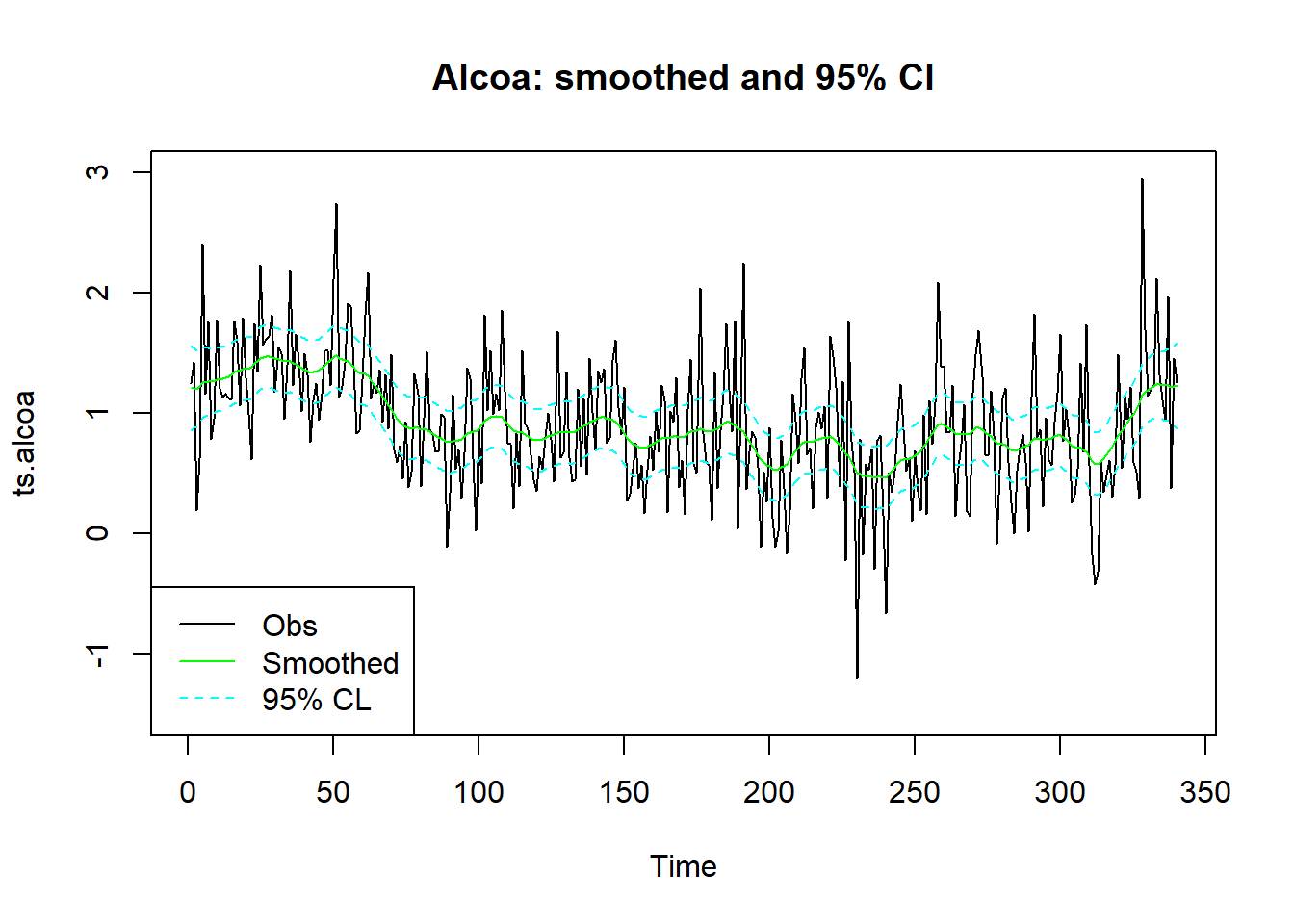

28.3.1.2 用KFAS

下面改用KFAS包进行估计。这个包也支持对结构时间序列模型进行简化的模型设定。

library(KFAS)
## 模型设定
kfas01a <- SSModel(
  ts.alcoa ~ SSMtrend(
    1, Q=list(matrix(NA))), 
  H=matrix(NA))
## 超参数估计
kfas01b <- fitSSM(
  kfas01a, 
  rep(log(var(ts.alcoa)), 2), 
  method="BFGS")
c("Var_obs"=c(kfas01b$model$H), 
  "Var_level"=c(kfas01b$model$Q))

##     Var_obs   Var_level 
## 0.230651733 0.005404091

## 用估计的超参数进行滤波平滑
kfas01c <- KFS(kfas01b$model)

超参数估计结果与statespacer基本一致。计算两个包的平滑结果的最大差距：

c("水平值平滑差距"=max(abs(
  c(ssr1$smoothed$level) - c(kfas01c$muhat))),
  "水平值平滑方差差距"=max(abs(
    c(ssr1$smoothed$V) - c(kfas01c$V_mu))))

##     水平值平滑差距 水平值平滑方差差距 
##       3.475598e-05       9.103878e-07

可见statespacer和KFAS两个包的平滑结果是一致的。

28.3.1.3 用dlm

dlm包也可以实现这个模型。在超参数\(\sigma_e^2\)和\(\sigma_{\eta}^2\)已知时，可以指定模型如下：

library(dlm)
dlm(
  FF = 1,  # $Z_t$矩阵
  V = 0.8, # $\sigma_e^2$
  GG = 1,  # $T_t$矩阵
  W = 0.1, # $\sigma_{\eta}^2$
  m0 = 0,  # 与$a_1$作用相同，为$\mu_0$期望
  C0 = 100 # 与$P_1$作用相同，为$\mu_0$方差
)

## $FF
##      [,1]
## [1,]    1
## 
## $V
##      [,1]
## [1,]  0.8
## 
## $GG
##      [,1]
## [1,]    1
## 
## $W
##      [,1]
## [1,]  0.1
## 
## $m0
## [1] 0
## 
## $C0
##      [,1]
## [1,]  100

也可以用dlmModPoly()指定这样的局部水平模型：

dlmModPoly(
  order = 1,  # 局部水平模型
  dV = 0.8, # $\sigma_e^2$
  dW = 0.1, # $\sigma_{\eta}^2$
  C0 = 100 # 与$P_1$作用相同，为$\mu_0$方差
)

## $FF
##      [,1]
## [1,]    1
## 
## $V
##      [,1]
## [1,]  0.8
## 
## $GG
##      [,1]
## [1,]    1
## 
## $W
##      [,1]
## [1,]  0.1
## 
## $m0
## [1] 0
## 
## $C0
##      [,1]
## [1,]  100

为了对超参数进行最大似然估计，需要自定义一个给定超参数后输出dlm模型的函数：

buildFun <- function(para){
  dlmModPoly(
    order = 1,
    dV = exp(para[[1]]),
    dW = exp(para[[2]])
  )
}

注意模型中并没有输入数据。用dlmMLE()函数输入数据后对超参数进行最大似然估计：

fit_dlm <- dlmMLE(
  ts.alcoa,       # 输入的观测值序列
  parm = c(0, 0), # 超参数对数值的初值
  build = buildFun
)
fit_dlm$conv

## [1] 0

获得估计的超参数对应的dlm模型：

dlm_al <- buildFun(fit_dlm$par)

估计的超参数值：

c("Var_obs" = dlm::V(dlm_al), 
  "Var_level" = dlm::W(dlm_al))

##    Var_obs  Var_level 
## 0.23065283 0.00540346

估计结果与statespacer和KFAS结果基本相同。为了获得滤波结果，可以调用dlmFilter(dlm_al)，平滑结果使用dlmSmooth(dlm_al)，从结果中可以很容易地提取滤波估计与平滑估计，但是条件分布方差阵估计使用了奇异值分解表示，提取时要使用dlmSvd2var()函数转换为方差阵。

28.3.1.4 用MARSS

局部水平模型写成MARSS需要的形式为： \[\begin{aligned} x_t =&\ 1 \cdot x_{t-1} + 0 + w_t, && w_t \sim \text{N}(0, q), \\ y_t =&\ 1 \cdot x_t + 0 + v_t, && r_t \sim \text{N}(0, r), \\ x_0 =&\ \mu . \end{aligned}\]

估计：

library(MARSS)
fit_marss_al <- MARSS(ts.alcoa, model=list(
  B = "identity", 
  U = "zero", 
  Q = matrix("q"), 
  Z = "identity", 
  A = "zero", 
  R = matrix("r"), 
  x0 = matrix("mu")) )

## Success! abstol and log-log tests passed at 132 iterations.
## Alert: conv.test.slope.tol is 0.5.
## Test with smaller values (<0.1) to ensure convergence.
## 
## MARSS fit is
## Estimation method: kem 
## Convergence test: conv.test.slope.tol = 0.5, abstol = 0.001
## Estimation converged in 132 iterations. 
## Log-likelihood: -258.2761 
## AIC: 522.5521   AICc: 522.6235   
##  
##       Estimate
## R.r    0.22958
## Q.q    0.00567
## x0.mu  1.20767
## Initial states (x0) defined at t=0
## 
## Standard errors have not been calculated. 
## Use MARSSparamCIs to compute CIs and bias estimates.

两个方差的估计与statespacer结果相近，不完全相同。

状态的平滑结果用tsSmooth(object, type="xtT")提取，均值为.estimate，标准误差为.se。如：

plot(ts.alcoa, main="Alcoa LL smoothing using MARSS")
res_sm <- tsSmooth(fit_marss_al, type="xtT")
lines(res_sm$.estimate,
  col = "red")
lines(res_sm$.estimate - 1.96*res_sm$.se,
  col = "green", lty=3)
lines(res_sm$.estimate + 1.96*res_sm$.se,
  col = "green", lty=3)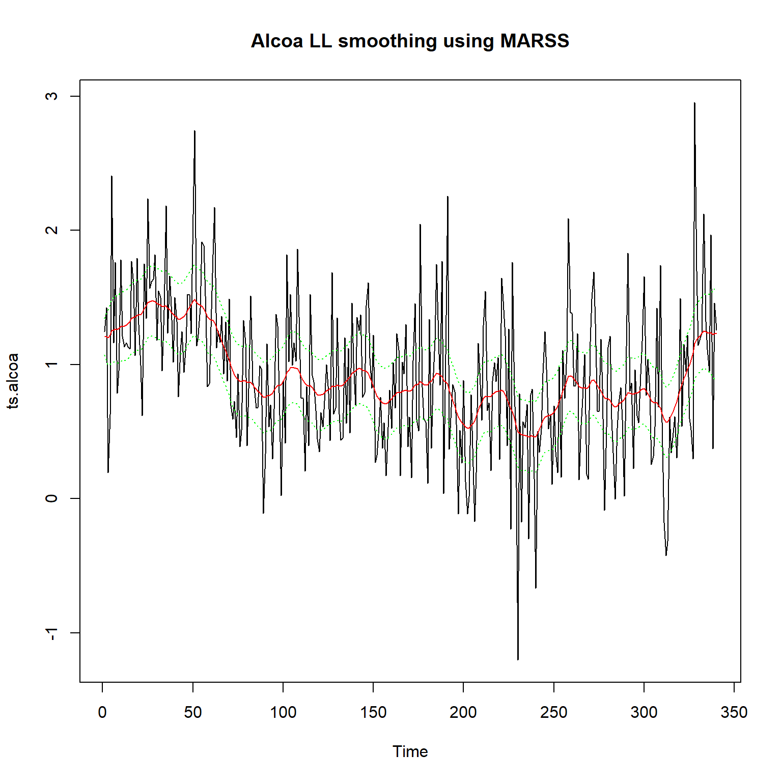

28.3.2 尼罗河流量带变点的局部水平模型

例28.5 考虑尼罗河1871-1970年的年流量数据，单位是\(10^8\)立方米，在1898-1899年有明显的变点。用局部水平模型建模并考虑变点的拟合。

基本R的datasets包中Nile变量为长度100的时间序列：

plot(Nile, main="Annual flow of Nile")
abline(v = c(1898, 1899), lty=3, col="yellow")

28.3.2.1 用DLM包

使用dlm包，输入超参数建立dlm模型的函数：

library(dlm)
buildFun <- function(para){
  mod <- dlmModPoly(
    order = 1,
    dV = exp(para[[1]]) # $\sigma_e^2$，非时变  
  )
  mod$JW <- matrix(1)   # 示性函数，表示$\sigma_{\eta_t}^2$时变
  # mod$X: 用来保存时变的成分
  mod$X <- cbind(rep(exp(para[[2]]), length(Nile)))
  # 给t=1898年的观测的$\eta_t$方差放大
  jj <- which(time(Nile) == 1899)[1]
  mod$X[jj,1] <- mod$X[jj,1] * (1 + exp(para[[3]]))
  
  mod
}

在上面的模型中，状态方差的扰动项\(\eta_t\)的方差是时变的，但仅在1899年与其它年份不同。为了容许模型中的矩阵时变，在dlm中用JW作为示性函数，表示状态方程的扰动项方差阵哪些元素是时变的，然后将时变的内容保存在X矩阵中，矩阵的行数等于观测长度\(n\)。用第三个超参数表示1899年的状态方程扰动项方差放大倍数（对数尺度）。

三个超参数的最大似然估计：

fit_nile <- dlmMLE(
  Nile,
  parm = c(0, 0, 0), 
  build = buildFun)
fit_nile$conv

## [1] 0

获取估计的模型：

dlm_nile <- buildFun(fit_nile$par)

\(\sigma_e^2\)估计：

V(dlm_nile)

##          [,1]
## [1,] 16300.33

除去变点以外的所有观测的\(\eta_t\)方差估计，以及1899年的\(\eta_t\)方差估计：

dlm_nile$X[c(1, which(time(Nile) == 1899)[1]), 1]

## [1] 2.792224e-02 6.048379e+04

可以看出，非变点处的\(\eta_t\)的标准差，与观测\(y_t\)的取值范围相比，基本上等于0。

计算滤波和平滑估计：

filt_nile <- dlmFilter(Nile, dlm_nile)
sm_nile <- dlmSmooth(filt_nile)

提取平滑估计：

sme_nile <- dropFirst(sm_nile$s)

提取平滑分布方差：

smv_nile <- dlmSvd2var(sm_nile$U.S, sm_nile$D.S) |> 
  unlist() |>
  dropFirst()

作原始序列图，添加平滑结果曲线（红色），平滑区间（绿色）：

plot(Nile, type="o", main="Smoothed Nile Flow")
lines(sme_nile, col="red")
lines(sme_nile - 1.96 * sqrt(smv_nile), lty=3, col="green")
lines(sme_nile + 1.96 * sqrt(smv_nile), lty=3, col="green")
abline(v=c(1898, 1899), lty=3, col="yellow")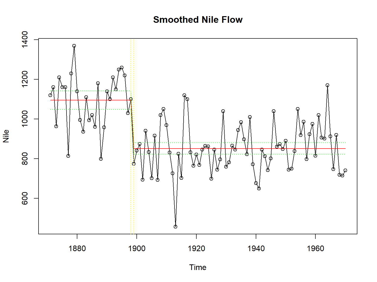

这个模型中的\(\eta_t\)的方差是时变的，水平在1898到1999之间有一个变点，在变化之前的\(\eta_t\)的方差基本恒定，水平也基本恒定，变化之后也是如此。

○○○○○

28.3.2.2 用MARSS包

为了演示MARSS的用法，先考虑一个恒定水平模型： \[ y_t = a + \nu_t, \ \nu_t \sim \text{N}(0, R) . \] 将其写成MARSS需要的形式： \[\begin{aligned} x_t =& 1 \times x_{t-1} + 0 + w_t, \ w_t \sim \text{N}(0, 0), \\ y_t =& 1 \times x_t + 0 + \nu_t, \ \nu_t \sim \text{N}(0, R), \\ x_0 =& a . \end{aligned}\] 因为\(x_0=a\)，\(w_t = a\)，所以\(x_t \equiv a\)，不需要估计变化的\(x_t\)。程序可以写成

library(MARSS)
fit1_mn <- MARSS(Nile, model = list(
  B = "identity", 
  U = "zero", 
  Q = "zero", 
  Z = "identity", 
  A = "zero", 
  R = matrix("r"), 
  x0 = matrix("a")) )

## Success! algorithm run for 15 iterations. abstol and log-log tests passed.
## Alert: conv.test.slope.tol is 0.5.
## Test with smaller values (<0.1) to ensure convergence.
## 
## MARSS fit is
## Estimation method: kem 
## Convergence test: conv.test.slope.tol = 0.5, abstol = 0.001
## Algorithm ran 15 (=minit) iterations and convergence was reached. 
## Log-likelihood: -654.5157 
## AIC: 1313.031   AICc: 1313.155   
##  
##      Estimate
## R.r     28352
## x0.a      919
## Initial states (x0) defined at t=0
## 
## Standard errors have not been calculated. 
## Use MARSSparamCIs to compute CIs and bias estimates.

然后，考虑趋势为非随机直线的模型。即 \[ y_t = a + ut + \nu_t . \] 写成MARSS标准形式： \[\begin{aligned} x_t =& 1 \times x_{t-1} + u + w_t, \ w_t \sim \text{N}(0, 0), \\ y_t =& 1 \times x_t + 0 + \nu_t, \ \nu_t \sim \text{N}(0, R), \\ x_0 =& a . \end{aligned}\] 程序为

fit2_mn <- MARSS(Nile, model = list(
  B = "identity", 
  U = matrix("u"), 
  Q = "zero", 
  Z = "identity", 
  A = "zero", 
  R = matrix("r"), 
  x0 = matrix("a")) )

## Success! abstol and log-log tests passed at 18 iterations.
## Alert: conv.test.slope.tol is 0.5.
## Test with smaller values (<0.1) to ensure convergence.
## 
## MARSS fit is
## Estimation method: kem 
## Convergence test: conv.test.slope.tol = 0.5, abstol = 0.001
## Estimation converged in 18 iterations. 
## Log-likelihood: -642.3159 
## AIC: 1290.632   AICc: 1290.882   
##  
##      Estimate
## R.r  22213.60
## U.u     -2.69
## x0.a  1054.94
## Initial states (x0) defined at t=0
## 
## Standard errors have not been calculated. 
## Use MARSSparamCIs to compute CIs and bias estimates.

拟合不考虑变点的局部水平模型。 MARSS模型公式为 \[\begin{aligned} x_t =& 1 \times x_{t-1} + 0 + w_t, \ w_t \sim \text{N}(0, Q), \\ y_t =& 1 \times x_t + 0 + \nu_t, \ \nu_t \sim \text{N}(0, R), \\ x_0 =& x_0 . \end{aligned}\]

为了得到更精确的结果，可以在用EM估计后，用估计结果作为初值，使用BFGS算法估计：

fit3_mn_em <- MARSS(Nile, model = list(
  B = "identity", 
  U = "zero", 
  Q = matrix("q"), 
  Z = "identity", 
  A = "zero", 
  R = matrix("r"), 
  x0 = matrix("x0")) )

## Success! abstol and log-log tests passed at 74 iterations.
## Alert: conv.test.slope.tol is 0.5.
## Test with smaller values (<0.1) to ensure convergence.
## 
## MARSS fit is
## Estimation method: kem 
## Convergence test: conv.test.slope.tol = 0.5, abstol = 0.001
## Estimation converged in 74 iterations. 
## Log-likelihood: -637.7631 
## AIC: 1281.526   AICc: 1281.776   
##  
##       Estimate
## R.r      15066
## Q.q       1425
## x0.x0     1112
## Initial states (x0) defined at t=0
## 
## Standard errors have not been calculated. 
## Use MARSSparamCIs to compute CIs and bias estimates.

fit3_mn <- MARSS(Nile, model = list(
  B = "identity", 
  U = "zero", 
  Q = matrix("q"), 
  Z = "identity", 
  A = "zero", 
  R = matrix("r"), 
  x0 = matrix("x0")),
  inits = fit3_mn_em$par, 
  method = "BFGS")

## Success! Converged in 10 iterations.
## Function MARSSkfas used for likelihood calculation.
## 
## MARSS fit is
## Estimation method: BFGS 
## Estimation converged in 10 iterations. 
## Log-likelihood: -637.7451 
## AIC: 1281.49   AICc: 1281.74   
##  
##       Estimate
## R.r      15337
## Q.q       1218
## x0.x0     1112
## Initial states (x0) defined at t=0
## 
## Standard errors have not been calculated. 
## Use MARSSparamCIs to compute CIs and bias estimates.

下面考虑随机漂移项中带有一个非时变的漂移项的模型。这只要添加\(U\)为待估参数：

fit4_mn <- MARSS(Nile, model = list(
  B = "identity", 
  U = matrix("u"), 
  Q = matrix("q"), 
  Z = "identity", 
  A = "zero", 
  R = matrix("r"), 
  x0 = matrix("mu")) )

## Success! abstol and log-log tests passed at 94 iterations.
## Alert: conv.test.slope.tol is 0.5.
## Test with smaller values (<0.1) to ensure convergence.
## 
## MARSS fit is
## Estimation method: kem 
## Convergence test: conv.test.slope.tol = 0.5, abstol = 0.001
## Estimation converged in 94 iterations. 
## Log-likelihood: -637.3027 
## AIC: 1282.605   AICc: 1283.026   
##  
##       Estimate
## R.r   15585.28
## U.u      -3.25
## Q.q    1088.99
## x0.mu  1124.04
## Initial states (x0) defined at t=0
## 
## Standard errors have not been calculated. 
## Use MARSSparamCIs to compute CIs and bias estimates.

按AIC比较，增加漂移项并没有改善。

带有随机漂移项的模型，即具有随机斜率项的模型： \[\begin{aligned} y_t =& (1, 0) \begin{pmatrix} x_t \\ u_t \end{pmatrix} + \nu_t, \ \nu_t \sim \text{N}(0, R), \\ \begin{pmatrix} x_t \\ u_t \end{pmatrix} =& \begin{pmatrix} 1 & 1 \\ 0 & 1 \end{pmatrix} \begin{pmatrix} x_{t-1} \\ u_{t-1} \end{pmatrix} + \begin{pmatrix} w_t \\ z_t \end{pmatrix}, \ \begin{pmatrix} w_t \\ z_t \end{pmatrix} \sim \text{N}(0, \text{diag}(Q, P)) , \\ \begin{pmatrix} x_0 \\ u_0 \end{pmatrix} =& \begin{pmatrix} x_0 \\ u_0 \end{pmatrix} . \end{aligned}\] 程序为（为了算法收敛先指定初值用EM粗略估计，然后用BFGS估计）：

mod5 <- list(
  B = rbind(c(1,1), 
            c(0,1)), 
  U = "zero", 
  Q = ldiag(c("q", "p")),
  Z = rbind(c(1, 0)),
  A = "zero", 
  R = matrix("r"), 
  x0 = cbind(c("x0", "u0")))
fit5_mn_tmp <- MARSS(Nile, model = mod5,
  inits = list(x0 = cbind(c(1000, -4))),
  control = list(maxit = 20),
  silent = TRUE)
fit5_mn <- MARSS(Nile, model = mod5,
  inits = fit5_mn_tmp,
  method = "BFGS")

## Success! Converged in 86 iterations.
## Function MARSSkfas used for likelihood calculation.
## 
## MARSS fit is
## Estimation method: BFGS 
## Estimation converged in 86 iterations. 
## Log-likelihood: -637.278 
## AIC: 1284.556   AICc: 1285.194   
##  
##        Estimate
## R.r    1.61e+04
## Q.q    8.43e+02
## Q.p    3.69e-07
## x0.x0  1.12e+03
## x0.u0 -3.11e+00
## Initial states (x0) defined at t=0
## 
## Standard errors have not been calculated. 
## Use MARSSparamCIs to compute CIs and bias estimates.

估计结果中随机斜率项的方差近似为0，所以斜率项实际是常数，从AIC看模型没有改善。

为了拟合1898-1899年的变点，考虑1899年的系统方程方差很大的模型。为了模型中的矩阵时变，需要使用三维数组，将时间\(t\)作为第三维。如：

jj <- which(time(Nile) == 1899)[1]
Q1 <- array("q", dim=c(1,1, length(Nile)))
Q1[1,1,jj] <- "q2"
y1 <- Nile / 1000
mod_list <-  list(
  B = "identity", 
  U = "zero", 
  Q = Q1, 
  Z = "identity", 
  A = "zero", 
  R = matrix("r"), 
  x0 = matrix("mu"))
fit6 <- MARSS(y1, 
  model = mod_list,
  control = list(maxit = 1000))

## Warning! Abstol convergence only. Maxit (=1000) reached before log-log convergence.
## 
## MARSS fit is
## Estimation method: kem 
## Convergence test: conv.test.slope.tol = 0.5, abstol = 0.001
## WARNING: Abstol convergence only no log-log convergence.
##  maxit (=1000) reached before log-log convergence.
##  The likelihood and params might not be at the ML values.
##  Try setting control$maxit higher.
## Log-likelihood: 61.58321 
## AIC: -115.1664   AICc: -114.7454   
##  
##       Estimate
## R.r   1.61e-02
## Q.q   3.58e-06
## Q.q2  6.13e-02
## x0.mu 1.10e+00
## Initial states (x0) defined at t=0
## 
## Standard errors have not been calculated. 
## Use MARSSparamCIs to compute CIs and bias estimates.
## 
## Convergence warnings
##  Warning: the  Q.q  parameter value has not converged.
##  Type MARSSinfo("convergence") for more info on this warning.

sm <- tsSmooth(fit6, type="xtT")
plot(y1, main="Nile smoothed with MARSS")
lines(as.vector(time(Nile)), sm$.estimate, col="red")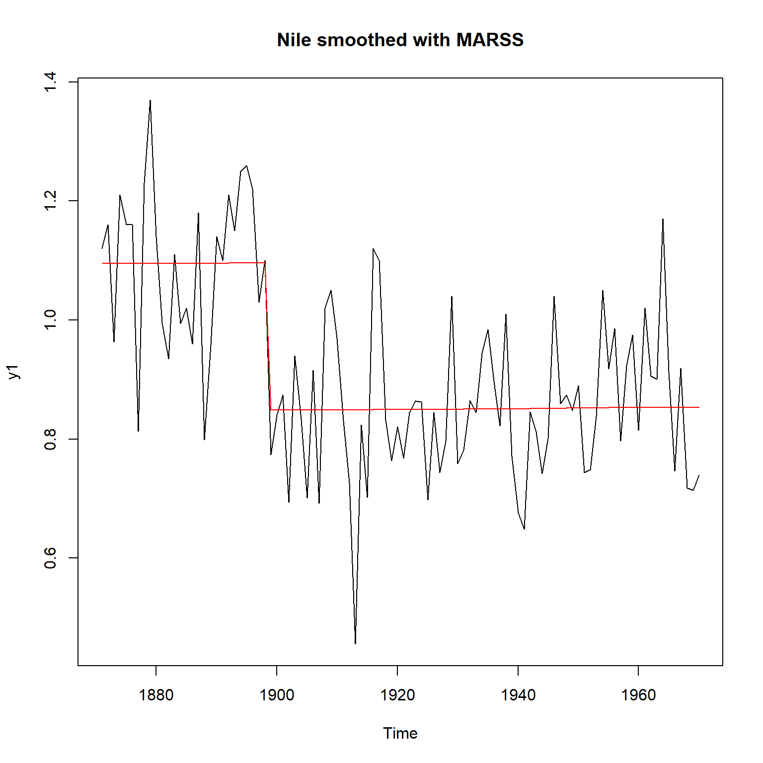

从AIC值比较，这个模型比前面的模型要好得多。系统方程在变点以外的误差项方差基本等于零。

MARSS包与DLM包得到的变点处的系统方程方差不同，这是因为只有一个变点，其方差估计本身就变化很大。

MARSS默认使用EM算法估计超参数，这种算法常常比较慢。一种方法是先用EM算法获得初步估计，然后使用BFGS等算法加速计算。

28.3.3 英国燃气消耗量结构时间序列建模

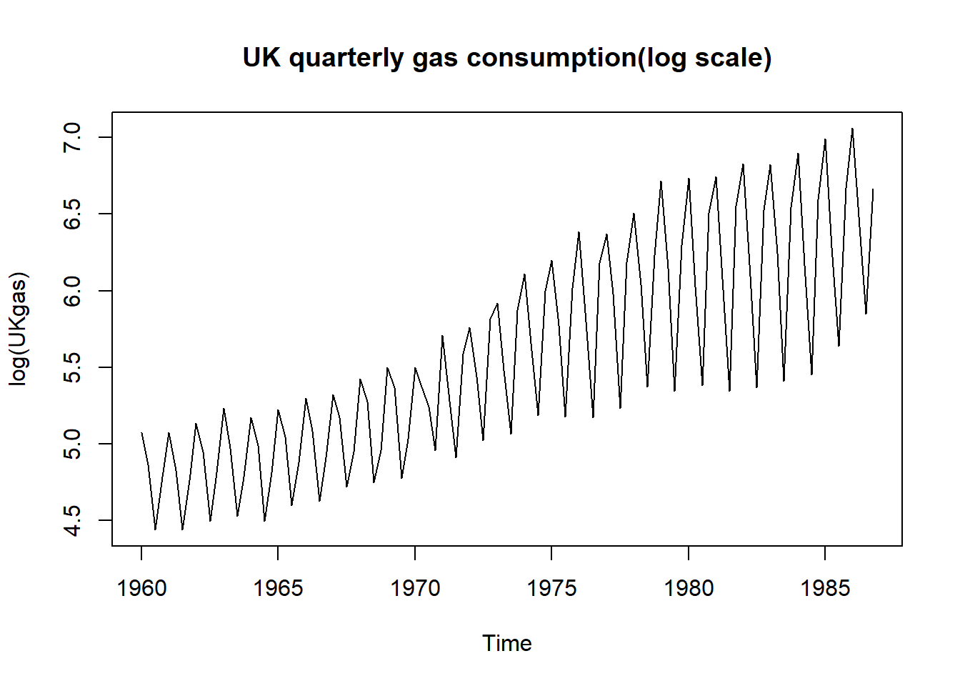
基本R的datasets包的UKgas变量保存了英国1960年到1986年的季度燃气消耗时间序列。使用结构时间序列建模，需要有趋势部分和季节部分。

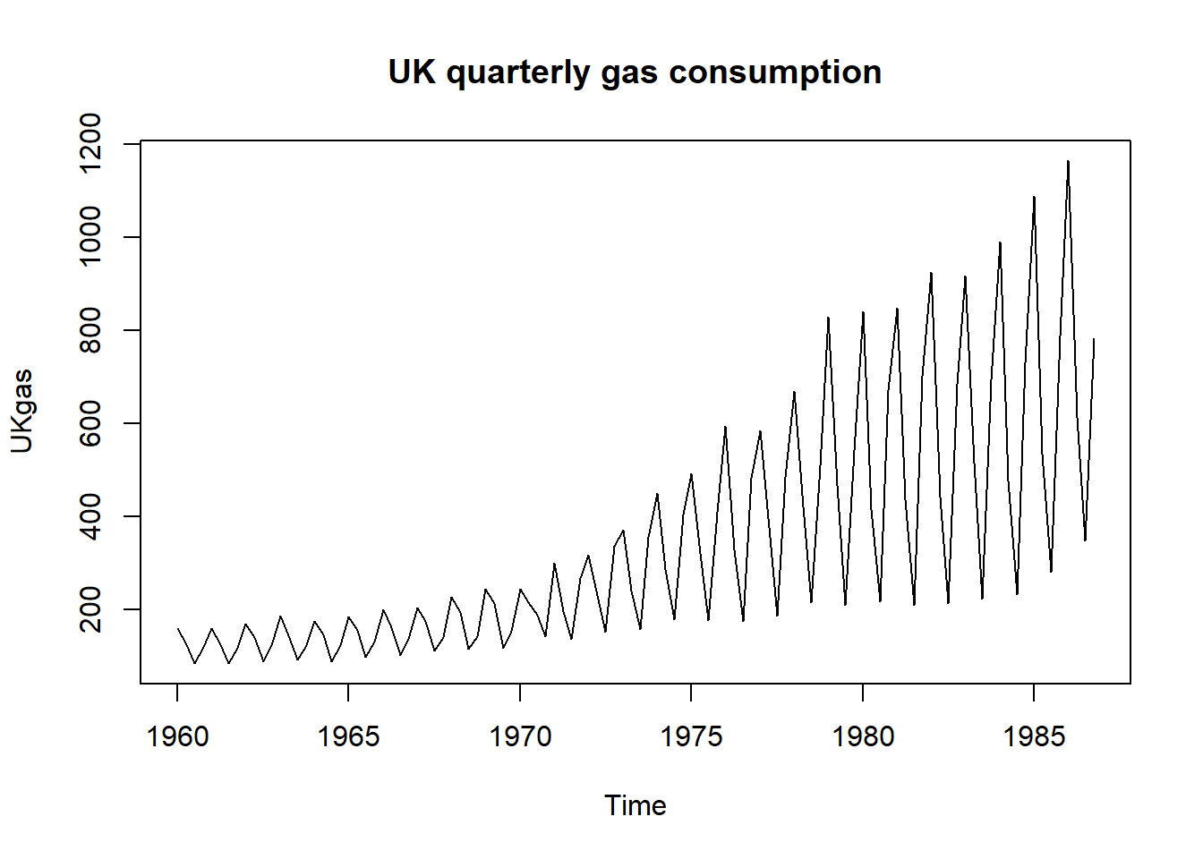
plot(UKgas, main="UK quarterly gas consumption")

因为趋势与季节部分呈现乘性的组合，改用对数值：

plot(log(UKgas), main="UK quarterly gas consumption(log scale)")

28.3.3.1 用dlm包

dlm包支持结构时间序列模型的简单设定。

指定模型：

library(dlm)
lGas <- log(UKgas)
dlmGas <- dlmModPoly() + dlmModSeas(4)

函数dlmModPoly()会指定一个有局部水平和水平的增量（时变斜率）的模型， dlmModSeas(4)指定季节模型，用加号表示这两部分的状态分别建模，在观测方程中将两部分结果相加。

拟合模型：

buildFun <- function(para){
  dlmGas <- dlmModPoly() + dlmModSeas(4)
  # 仅指定了时变斜率和季节项的方差，
  # 没有指定局部水平的方差
  diag(W(dlmGas))[2:3] <- exp(para[1:2])
  V(dlmGas) <- exp(para[3])
  
  dlmGas
}
fit_gas <- dlmMLE(
  lGas,
  parm = log(c(10^-5, 10^-3, 10^-3)), 
  build = buildFun )
fit_gas$conv

## [1] 0

估计得到的模型：

dlmGas <- buildFun(fit_gas$par)

观测方程方差：

drop(V(dlmGas))

## [1] 0.001822492

状态方程方差：

diag(W(dlmGas))[2:3]

## [1] 7.901263e-06 3.308590e-03

获取平滑得到的水平、季节项：

sm_gas <- dlmSmooth(lGas, mod=dlmGas)
da_tmp <- cbind(
  lGas,
  dropFirst(sm_gas$s[, c(1,3)]))
colnames(da_tmp) <- c("Gas", "Trend", "Seasonal")
plot(da_tmp, type="o", 
  main = "UK gas consumption structral model")

预报分布的均值和方差可以用dlmForecast()获得。下面的预测区间是\(90\%\)置信度的。

filt_gas <- dlmFilter(lGas, mod = dlmGas)
fore_gas <- dlmForecast(filt_gas, nAhead = 20)
# 预测
gas_pred20 <- fore_gas$f[,1]
gas_se20 <- sqrt(unlist(fore_gas$Q))
da_tmp <- ts.union(
  window(lGas, start=c(1982,1)),
  window(sm_gas$s[,1] + sm_gas$s[,3], start=c(1982,1)),
  gas_pred20,
  gas_pred20 - 1.96 * gas_se20, 
  gas_pred20 + 1.96 * gas_se20)
plot(da_tmp, plot.type = "single",
  type = "o", 
  pch = c(1, 2, 20, 3, 3),
  col = c("darkgrey", "green", 
    "brown", "yellow", "yellow"),
  ylab = "Gas consumption prediction"
  )

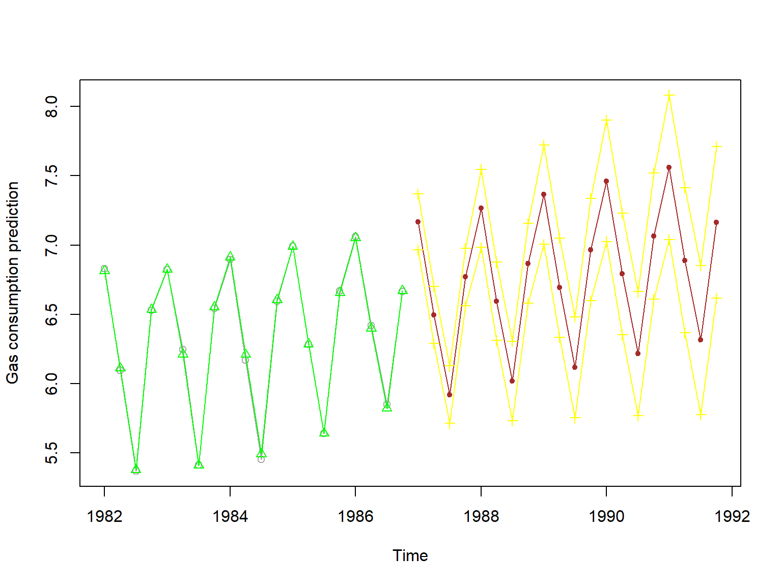
绿色三角形部分是平滑结果，其中黑色圆圈是真实值；棕色部分是多步预测结果，黄色是95%预测区间。

使用dlm发现，如果在dlmMLE()中使用parm=rep(0, 3)，则将原始数据作自然对数变换的结果比较好，状态方程扰动方差和观测方程扰动方差很小，但改为常用对数变换时，状态方程扰动项方差会增大一两个数量级，使得上图中的预测区间会大得不可接受。如果在dlmMLE()中人为取parm为较合适的初值，就可以得到与自然对数变换相同的结果，这说明dlm计算最大似然估计可能不太可靠，很可能落入局部极值点。 dlmMLE()的结果会依赖于参数的初始值parm的选择。

28.3.3.2 用MARSS

将季度数据的结构时间序列模型写成： \[\begin{aligned} \boldsymbol x_t =&\ \begin{pmatrix} \mu_t \\ \mu_t^{b} \\ \gamma_t \\ \gamma_{t-1} \\ \gamma_{t-2} \end{pmatrix} = \begin{pmatrix} 1 & 1 & 0 & 0 & 0 \\ 0 & 1 & 0 & 0 & 0 \\ 0 & 0 & -1& -1& -1 \\ 0 & 0 & 1 & 0 & 0 \\ 0 & 0 & 0 & 1 & 0 \end{pmatrix} \boldsymbol x_{-1} + \boldsymbol w_t, \\ &\ \boldsymbol w_t \sim \text{N}(\boldsymbol 0, \text{diag}(q_{\mu}, q_{\mu^b}, q_{\gamma}, 0)) \\ y_t =&\ (1, 0, 1, 0, 0) \boldsymbol x_t + \nu_t, \quad \nu_t \sim \text{N}(0, R) , \\ x_0 \sim&\ \text{N}(\mu_0, V_0) . \end{aligned}\]

制作这样的模型设定用列表：

build_sts4 <- function(y){
  B1 <- matrix(c(
    1, 1, 0, 0, 0,
    0, 1, 0, 0, 0,
    0, 0, -1,-1,-1,
    0, 0, 1, 0, 0,
    0, 0, 0, 1, 0 ),
    nrow = 5, byrow=TRUE)
  Q1 <- ldiag(list("qmu", "qmub", "qgam", 0, 0))

  Z1 <- rbind(c(1, 0, 1, 0, 0))
  R1 <- matrix("r")
  A1 <- matrix(0)
  
  x0 <- cbind(c(y[1], rep(0, 4)))
  vy <- var(y)/100
  ## 扩散先验
  #V0 <- matrix(vy*1E-6, 5, 5) + diag(1E-10, 5)
  V0 <- matrix(vy*1E6, 5, 5) + diag(1E-10, 5)

  list(
    B = B1,
    Q = Q1,
    Z = Z1,
    R = R1,
    U = "zero", 
    A = "zero", 
    x0 = x0, V0 = V0
    )
}

这里V0参数是\(\boldsymbol x_0\)的分布方差，这里指定了一个发散先验，即很大的方差。

建模：

library(MARSS)
gas_marss <- MARSS(lGas,
  model = build_sts4(lGas),
  method="BFGS")

## Success! Converged in 15 iterations.
## Function MARSSkfas used for likelihood calculation.
## 
## MARSS fit is
## Estimation method: BFGS 
## Estimation converged in 15 iterations. 
## Log-likelihood: 66.215 
## AIC: -124.43   AICc: -124.0417   
##  
##        Estimate
## R.r    4.49e-06
## Q.qmu  1.74e-03
## Q.qmub 3.62e-06
## Q.qgam 5.35e-03
## Initial states (x0) defined at t=0
## 
## Standard errors have not been calculated. 
## Use MARSSparamCIs to compute CIs and bias estimates.

带有季节成分的模型使用MARSS默认的EM算法往往比较困难，所以这里用了BFGS算法。

平滑结果：

sm <- fitted(gas_marss, type="ytT")
plot(lGas)
lines(as.vector(time(lGas)), sm$.fitted, col="red", lty=2)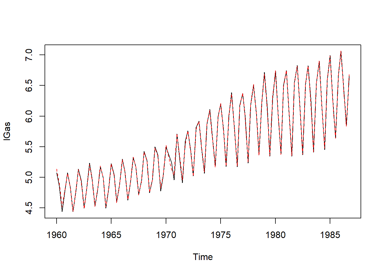

拟合误差很小，这也可以从估计的观测误差方差(R.r)远小于水平的误差方差(Q.qmu)解释。各个分解成分情况：

sm2 <- tsSmooth(gas_marss, type="xtT")
sm2t <- sm2 |>
  pivot_wider(
    id_cols = "t",
    names_from = ".rownames",
    values_from = ".estimate"  ) |>
  rename(level = X1, slope = X2, season = X3)
plot(ts(sm2t[,2:4], start=start(lGas), frequency=4),
  main="log(Gas) decomposition using MARSS")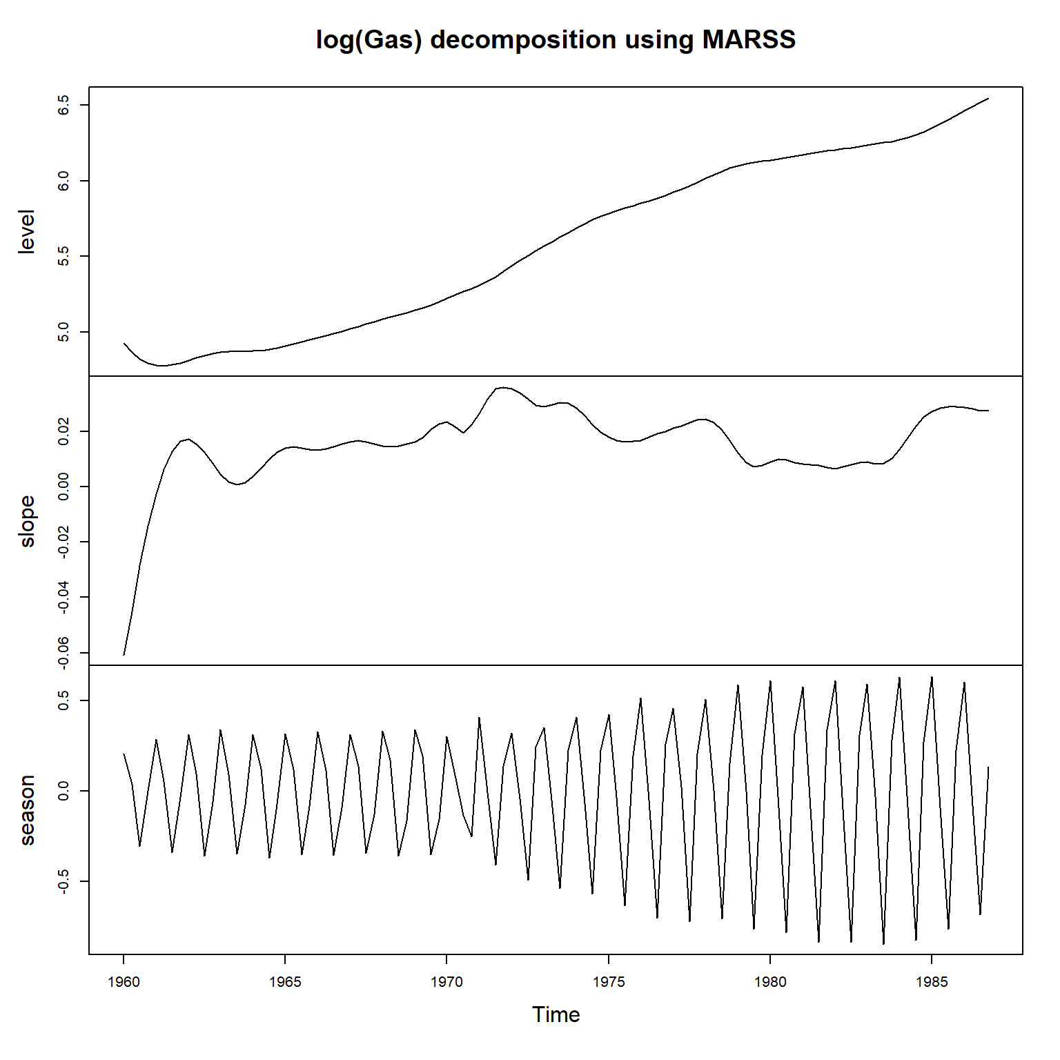

预测：

library(forecast)
gas_fore <- forecast(gas_marss, h=20, interval="prediction")
plot(gas_fore, showgap=FALSE)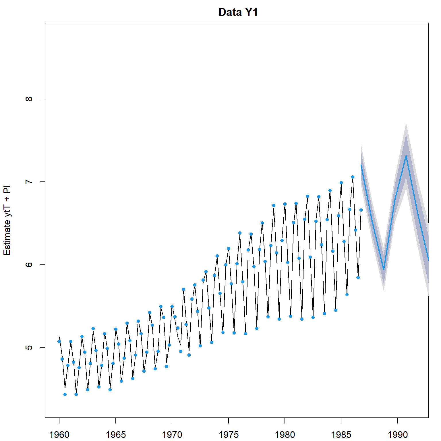

预测图形中深浅不同的阴影分别是80%和95%预测区间。所谓预测区间，就是考虑了观测误差的影响。

可以用residuals()提取估计残差。

28.4 ARMA和ARIMA模型

考虑ARMA(\(p,q\))模型，取\(r=\max(p,q+1)\)，则模型可以写成 \[ y_t = \sum_{j=1}^r \phi_j y_{t-j} + \zeta_t + \sum_{j=1}^{r-1} \theta_j \zeta_{t-j}, \] 其中某些系数可以为0。将此模型写成状态空间模型形式，有多种不同形式，这里给出一种形式比较复杂但计算方便的表达形式： \[\begin{aligned} \boldsymbol\alpha_t =& \begin{pmatrix} y_t & \\ \phi_2 y_{t-1} + \dots + \phi_r y_{t - (r-1)} & + \theta_1 \zeta_t + \dots + \theta_{r-1} \zeta_{t-(r-2)} \\ \phi_3 y_{t-1} + \dots + \phi_r y_{t - (r-2)} & + \theta_2 \zeta_t + \dots + \theta_{r-1} \zeta_{t-(r-3)} \\ \vdots & \vdots \\ \phi_r y_{t-1} & + \theta_{r-1} \zeta_t \end{pmatrix} \\ y_t =& (1, 0, 0, \dots, 0) \boldsymbol\alpha_t \\ \boldsymbol\alpha_{t+1} =& \begin{pmatrix} \phi_1 & 1 & 0 & \cdots & 0 \\ \phi_2 & 0 & 1 & \cdots & 0 \\ \vdots & \vdots & & \ddots & \vdots \\ \phi_{r-1} & 0 & 0 & \cdots & 1 \\ \phi_r & 0 & 0 & \cdots & 0 \end{pmatrix} \boldsymbol\alpha_t + \begin{pmatrix} 1 \\ \theta_1 \\ \theta_2 \\ \vdots \\ \theta_{r-1} \end{pmatrix} \zeta_{t+1} . \end{aligned}\]

对一个ARIMA(2,1,1)，模型 \[\begin{aligned} y_t^* =& y_t - y_{t-1}, \\ y_t^* =& \phi_1 y_{t-1}^* + \phi_2 y_{t-2}^* + \zeta_t + \theta_1 \zeta_{t-1}, \end{aligned}\] 可以写成 \[\begin{aligned} \boldsymbol\alpha_t =& \begin{pmatrix} y_{t-1} \\ y_t^* \\ \phi_2 y_{t-1}^* + \theta_1 \zeta_t \end{pmatrix} \\ y_t =& (1,1,0) \boldsymbol\alpha_t \\ \boldsymbol\alpha_{t+1} =& \begin{pmatrix} 1 & 1 & 0 \\ 0 & \phi_1 & 1 \\ 0 & \phi_2 & 0 \end{pmatrix} \boldsymbol\alpha_t + \begin{pmatrix} 0 \\ 1 \\ \theta_1 \end{pmatrix} \zeta_{t+1} \end{aligned}\] 观测方程没有观测误差。

更一般的ARIMA以及带有乘性季节部分的ARIMA都可以类似表示。将ARIMA模型表示成状态空间模型以后，好处是状态空间模型的一系列工具都可以用在ARIMA的模型推断中，比如SSM的精确最大似然估计和初始化方法都可以使用。现在的估计ARIMA模型的软件中许多都是利用状态空间模型形式进行估计和推断。

反过来，许多状态空间模型的观测值也服从ARIMA模型，比如局部趋势模型，带有斜率项的局部趋势模型等，加入了季节项的结构时间序列模型等。但是，结构时间序列模型转换成ARIMA模型会丢失一些有可解释含义的信息。

状态空间模型的优点：

状态空间模型更灵活，能够将随着时间增加的已知的机制变化添加到模型中，而ARIMA则很难修改；
容易处理缺失值；
很容易增加额外的解释变量，有回归自变量时允许回归系数为时变系数，很容易进行日历调整；
预测不需要单独的理论；
不要求平稳或者差分后平稳。

另一方面， ARIMA模型则无法将趋势成分、季节项成分提取出来，要求差分后平稳，而经济和金融中许多数据是差分后也不平稳的。

例28.6 考虑太阳黑子数的ARMA建模。数据为1700-1988的年数据。

数据：

library(datasets)
ts.ss <- window(sunspot.year, start = 1770, end = 1869)
plot(ts.ss)

可以看出，数据有周期性。

用R的arima函数建立AR(3)模型：

ss1 <- arima(
  ts.ss, order=c(3,0,0))
ss1

## 
## Call:
## arima(x = ts.ss, order = c(3, 0, 0))
## 
## Coefficients:
##          ar1      ar2     ar3  intercept
##       1.5471  -0.9915  0.2004    48.5119
## s.e.  0.0983   0.1545  0.0990     6.0560
## 
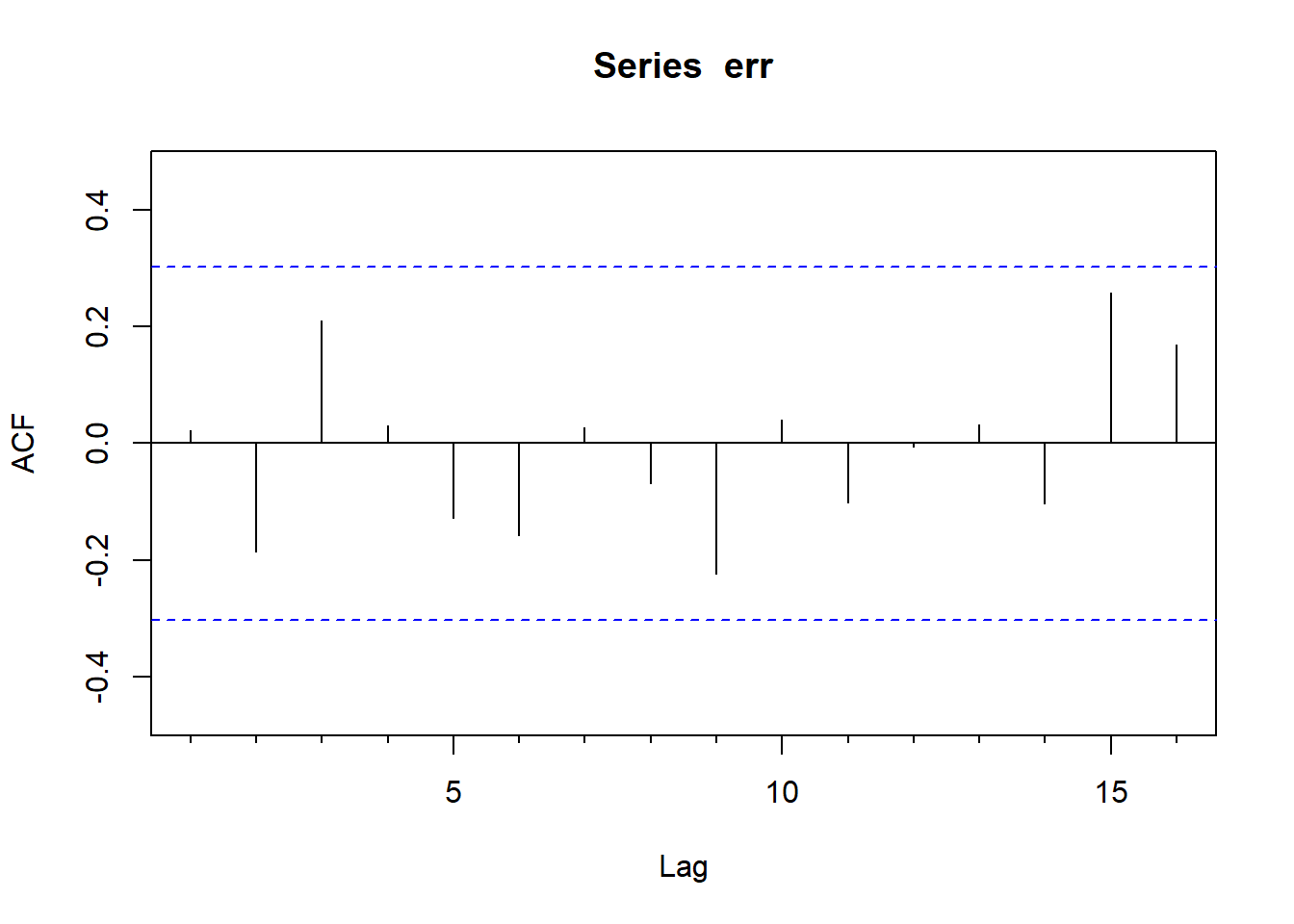
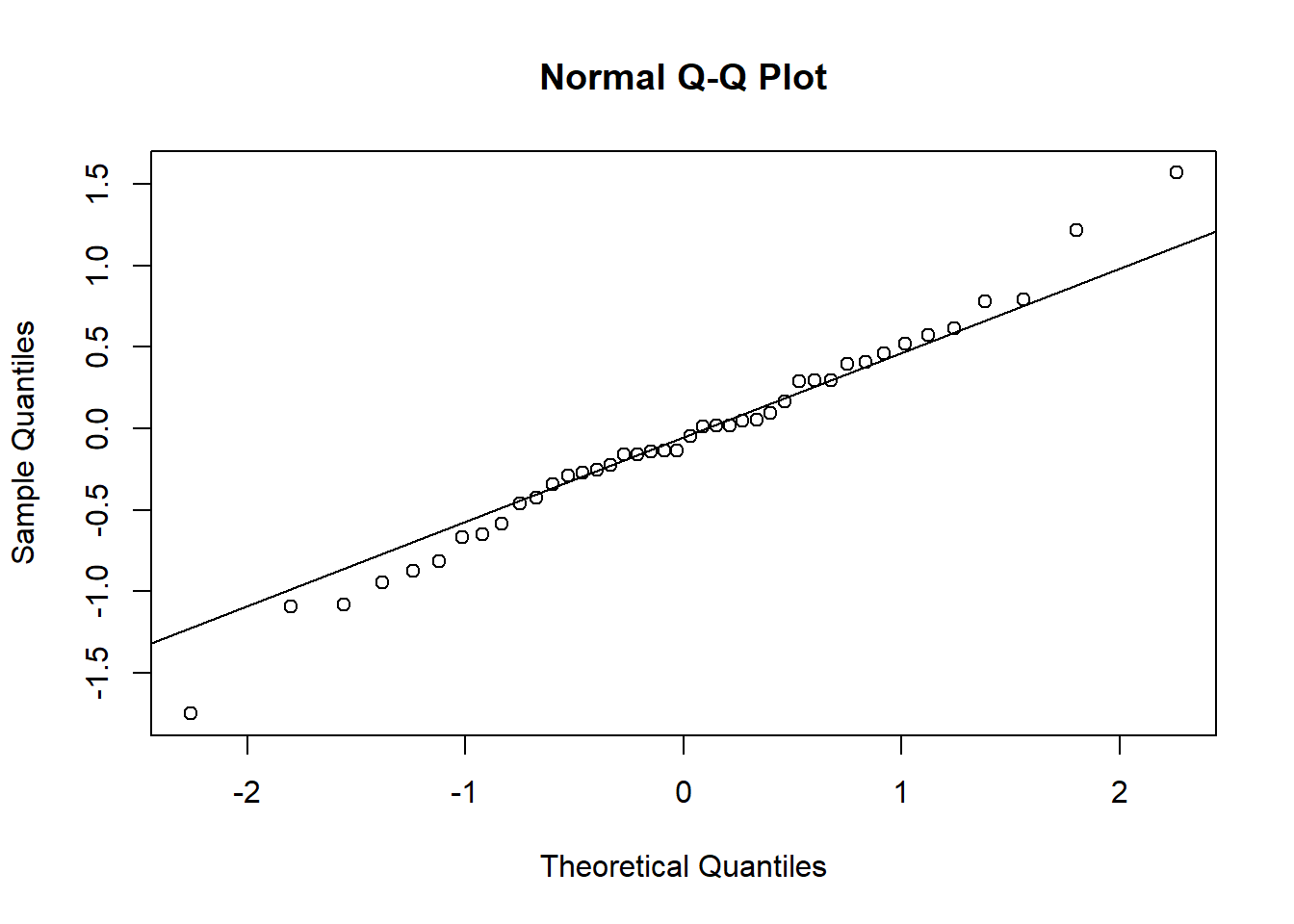
## sigma^2 estimated as 220.2:  log likelihood = -412.94,  aic = 835.88

估计的模型为 \[ (1 - 1.5471B + 0.9915B^2 - 0.2004B^3)(y_t - 48.5119) = e_t, \ e_t \sim \text{WN}(0, 220.2) . \] 模型诊断：

tsdiag(ss1)

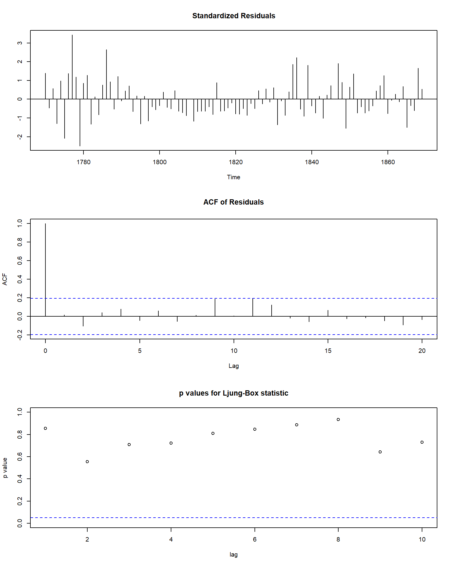
从模型诊断看是合适的。

估计的AR(3)中特征多项式的根和复根对应的周期：

rt1 <- polyroot(c(1, -coef(ss1)[1:3])); rt1

## [1] 1.045502+0.808659i 1.045502-0.808659i 2.855749-0.000000i

2*pi/Arg(rt1[1])

## [1] 9.543839

求出的周期9.5年左右，与实际观察到的大约11年周期不完全相同。

用statespacer包将AR(3)估计成状态空间模型，此包直接支持恢复ARIMA参数：

library(datasets)
library(statespacer)
mat.suns <- matrix(window(
  sunspot.year, start = 1770, end = 1869))
fit <- statespacer(
  y = mat.suns,
  H_format = matrix(0), 
  # H是观测方程的误差方差阵
  local_level_ind = TRUE,
  arima_list = list(c(3,0,0)),
  format_level = matrix(0),
  # format_level是结构时间序列模型中水平值$\mu_t$的方程的误差方差阵
  initial = c(0.5*log(var(mat.suns)), 0, 0, 0),
  verbose=TRUE)

## Starting the optimisation procedure at: 2023-05-26 09:26:40

## initial  value 5.022561 
## iter  10 value 4.114363
## final  value 4.111163 
## converged

## Finished the optimisation procedure at: 2023-05-26 09:26:40

## Time difference of 0.0616450309753418 secs

构造ARMA的结果：

arma_coeff <- rbind(
   fit$system_matrices$AR$ARIMA1,
   fit$standard_errors$AR$ARIMA1
)
arma_coeff <- cbind(
   arma_coeff,
   c(fit$smoothed$level[1],
     sqrt(fit$system_matrices$Z_padded$level %*%
          fit$smoothed$V[,,1] %*%
          t(fit$system_matrices$Z_padded$level))
   )
)
rownames(arma_coeff) <- c("coefficient", "std_error")
colnames(arma_coeff) <- c("ar1", "ar2", "ar3", "intercept")
arma_coeff

##                    ar1       ar2       ar3 intercept
## coefficient 1.55976415 -1.005462 0.2129622 48.605905
## std_error   0.09962468  0.155982 0.1003591  6.358039

与arima()函数结果相近但不完全相同。

例28.7 考虑航空乘客数的建模，1949-1961年的月度数据，用ARIMA\((0,1,1)(0,1,1)_{12}\)模型。

plot(AirPassengers)

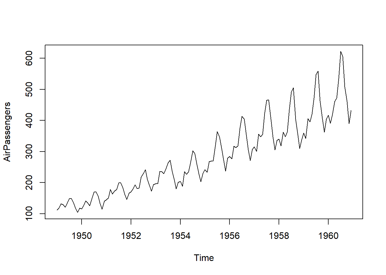
将数据取自然对数，用arima()建模：

ap01 <- arima(
  log(AirPassengers),
  order=c(0,1,1),
  seasonal=list(order=c(0,1,1), frequency=12))
ap01

## 
## Call:
## arima(x = log(AirPassengers), order = c(0, 1, 1), seasonal = list(order = c(0, 
##     1, 1), frequency = 12))
## 
## Coefficients:
##           ma1     sma1
##       -0.4018  -0.5569
## s.e.   0.0896   0.0731
## 
## sigma^2 estimated as 0.001348:  log likelihood = 244.7,  aic = -483.4

模型为： \[ (1 - B) (1 - B^{12}) \ln y_t = (1 - 0.4018B)(1 - 0.5569B^{12}) e_t, \ e_t \sim \text{WN}(0, 0.001348) . \]

利用statespacer计算：

mat.ap <- matrix(log(AirPassengers))

# 模型设定列表
sarima_list <- list(list(
  s = c(12, 1), ar = c(0, 0), i = c(1, 1), ma = c(1, 1) ))

# 拟合模型
fit <- statespacer(
  y = mat.ap,
  H_format = matrix(0),
  sarima_list = sarima_list,
  initial = c(0.5*log(var(diff(mat.ap))), 0, 0),
  verbose = TRUE)

## Starting the optimisation procedure at: 2023-05-26 09:26:40

## initial  value -1.034434 
## final  value -1.616321 
## converged

## Finished the optimisation procedure at: 2023-05-26 09:26:41

## Time difference of 0.461006164550781 secs

提取估计的参数：

arma_coeff <- rbind(
   c(fit$system_matrices$SMA$SARIMA1$S1,
     fit$system_matrices$SMA$SARIMA1$S12),
   c(fit$standard_errors$SMA$SARIMA1$S1,
     fit$standard_errors$SMA$SARIMA1$S12) )
rownames(arma_coeff) <- c("coefficient", "std_error")
colnames(arma_coeff) <- c("ma1 s = 1", "ma1 s = 12")
arma_coeff

##               ma1 s = 1  ma1 s = 12
## coefficient -0.40188859 -0.55694248
## std_error    0.08963614  0.07309788

goodness_fit <- rbind(
   fit$system_matrices$Q$SARIMA1,
   fit$diagnostics$loglik,
   fit$diagnostics$AIC
)
rownames(goodness_fit) <- c("Variance", "Loglikelihood", "AIC")
goodness_fit

##                        [,1]
## Variance        0.001347882
## Loglikelihood 232.750284785
## AIC            -3.010420622

结果与arima()结果相同。

28.5 回归模型

28.5.1 常系数回归模型

考虑回归模型 \[\begin{aligned} y_t = \boldsymbol X_t \boldsymbol\beta + e_t, \ e_t \sim \text{ iid N}(0, H_t), \ t=1,2,\dots,n , \end{aligned}\] 其中\(\boldsymbol X_t\)为\(1 \times k\)非随机的已知值， \(\boldsymbol\beta\)是\(k \times 1\)未知的回归系数向量。可以写成状态空间模型： \[\begin{aligned} \boldsymbol \alpha_t =& \boldsymbol\beta, \\ \boldsymbol\alpha_{t+1} =& I \boldsymbol\alpha_t, \\ y_t =& \boldsymbol X_t \boldsymbol\alpha_t + e_t . \end{aligned}\] 状态方程没有误差。

这个回归问题的加权最小二乘解为 \[\begin{aligned} \hat{\boldsymbol\beta} = (\sum_{i=1}^n \boldsymbol X_t^T H_t^{-1} \boldsymbol X_t)^{-1} \sum_{i=1}^n \boldsymbol X_t^T H_t^{-1} y_t . \end{aligned}\] 写成状态空间模型后，用滤波算法对\(\boldsymbol\alpha_t = \boldsymbol\beta\)进行估计，等价于对\(\boldsymbol\beta\)进行递推改进估计，相当于递推的最小二乘估计。

MARSS包的模型直接支持回归，其中的\(C_t \boldsymbol c_t\)是系统方程中的回归， \(\boldsymbol c_t\)是回归自变量数据； \(D_t \boldsymbol d_t\)是观测方程中的回归， \(\boldsymbol d_t\)是回归自变量数据。

对于常系数回归模型，因为回归系数不是时变的，这种模型可以用MARSS包的回归功能表示。仅进行回归的MARSS模型可以写成 \[\begin{aligned} x_0 =& 0 , \\ x_t =& 1 \times x_{t-1} + w_t, \ w_t \sim \text{N}(0, 0) \\ y_t =& 1 \times x_t + \beta d_t + v_t, \ v_t \sim \text{N}(0, Q). \end{aligned}\] 其中\(d_t\)是自变量在\(t\)时刻的观测值，如果有\(p\)个自变量，则\(c_t\)为\(p \times 1\)向量， \(\beta\)为\(1 \times p\)向量。

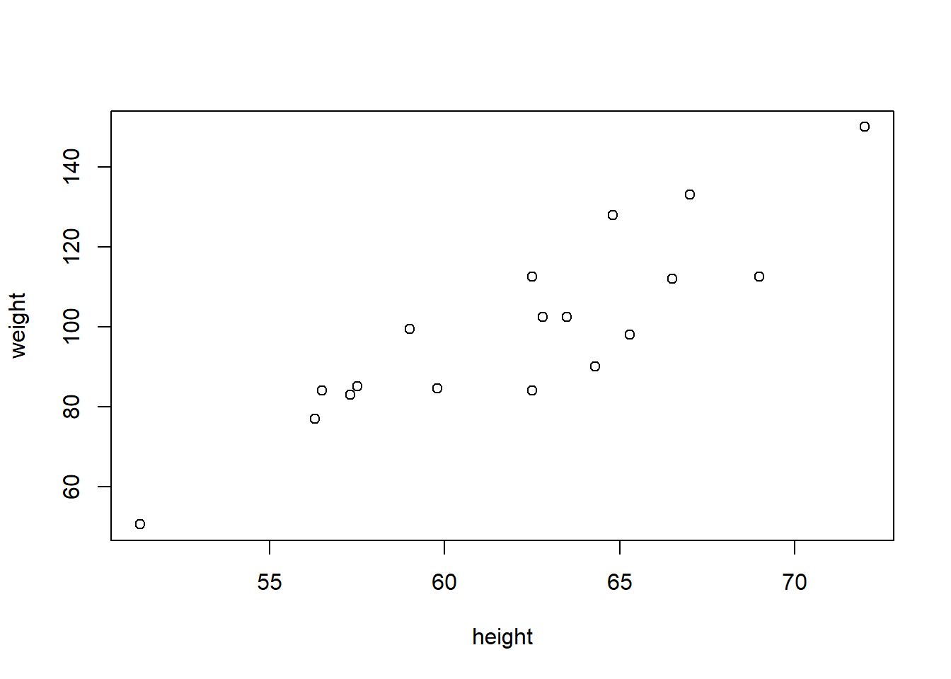
28.5.2 体重对身高的一元回归示例

考虑体重对身高的回归：

d_class <- readr::read_csv("class.csv",
  show_col_types = FALSE)
knitr::kable(d_class)

name	sex	age	height	weight
Alice	F	13	56.5	84.0
Becka	F	13	65.3	98.0
Gail	F	14	64.3	90.0
Karen	F	12	56.3	77.0
Kathy	F	12	59.8	84.5
Mary	F	15	66.5	112.0
Sandy	F	11	51.3	50.5
Sharon	F	15	62.5	112.5
Tammy	F	14	62.8	102.5
Alfred	M	14	69.0	112.5
Duke	M	14	63.5	102.5
Guido	M	15	67.0	133.0
James	M	12	57.3	83.0
Jeffrey	M	13	62.5	84.0
John	M	12	59.0	99.5
Philip	M	16	72.0	150.0
Robert	M	12	64.8	128.0
Thomas	M	11	57.5	85.0
William	M	15	66.5	112.0

with(d_class, plot(height, weight))

lm(weight ~ height, data=d_class) |>
  summary()

## 
## Call:
## lm(formula = weight ~ height, data = d_class)
## 
## Residuals:
##      Min       1Q   Median       3Q      Max 
## -17.6807  -6.0642   0.5115   9.2846  18.3698 
## 
## Coefficients:
##              Estimate Std. Error t value Pr(>|t|)    
## (Intercept) -143.0269    32.2746  -4.432 0.000366 ***
## height         3.8990     0.5161   7.555 7.89e-07 ***
## ---
## Signif. codes:  0 '***' 0.001 '**' 0.01 '*' 0.05 '.' 0.1 ' ' 1
## 
## Residual standard error: 11.23 on 17 degrees of freedom
## Multiple R-squared:  0.7705, Adjusted R-squared:  0.757 
## F-statistic: 57.08 on 1 and 17 DF,  p-value: 7.887e-07

用MARSS求解：

library(MARSS)
fit_class <- MARSS(
  rbind(d_class$weight), 
  model = list(
    B = "identity", 
    U = "zero", 
    Z = "identity",
    A = matrix("a"),
    x0 = "zero",
    Q = "zero",
    R = matrix("R"),
    D = matrix("beta"),
    d = rbind(d_class$height)))

## Success! algorithm run for 15 iterations. abstol and log-log tests passed.
## Alert: conv.test.slope.tol is 0.5.
## Test with smaller values (<0.1) to ensure convergence.
## 
## MARSS fit is
## Estimation method: kem 
## Convergence test: conv.test.slope.tol = 0.5, abstol = 0.001
## Algorithm ran 15 (=minit) iterations and convergence was reached. 
## Log-likelihood: -71.85003 
## AIC: 149.7001   AICc: 151.3001   
##  
##        Estimate
## A.a      -143.0
## R.R       112.8
## D.beta      3.9
## Initial states (x0) defined at t=0
## 
## Standard errors have not been calculated. 
## Use MARSSparamCIs to compute CIs and bias estimates.

与lm()估计结果基本相同。

不使用MARSS的回归功能，而是将回归写成普通的状态空间形式：

library(MARSS)
# 将输入矩阵的每行作为输出的三维数组的一个子矩阵
# 第三维代表时间$t$
row2d3 <- function(A){
  A <- t(A)
  dim(A) <- c(1, dim(A))
  A
}
fit_class2 <- MARSS(
  rbind(d_class$weight), model = list(
  B = "identity", 
  U = "zero", 
  Q = "zero",
  Z = row2d3(cbind(1, d_class$height)),
  A = "zero",
  x0 = cbind(c("beta0", "beta1")),
  R = matrix("R")),
  inits = list(x0=cbind(
    c(mean(d_class$weight),0))))

## Success! algorithm run for 15 iterations. abstol and log-log tests passed.
## Alert: conv.test.slope.tol is 0.5.
## Test with smaller values (<0.1) to ensure convergence.
## 
## MARSS fit is
## Estimation method: kem 
## Convergence test: conv.test.slope.tol = 0.5, abstol = 0.001
## Algorithm ran 15 (=minit) iterations and convergence was reached. 
## Log-likelihood: -71.85003 
## AIC: 149.7001   AICc: 151.3001   
##  
##          Estimate
## R.R         112.8
## x0.beta0   -143.0
## x0.beta1      3.9
## Initial states (x0) defined at t=0
## 
## Standard errors have not been calculated. 
## Use MARSSparamCIs to compute CIs and bias estimates.

28.5.3 变系数回归模型

考虑变系数的回归模型 \[\begin{aligned} y_t = \boldsymbol X_t \boldsymbol\beta_t + e_t, \ e_t \sim \text{ iid N}(0, H_t), \ t=1,2,\dots,n , \end{aligned}\] 其中的随时间而变化的回归系数可以用如下的随机游动建模： \[\begin{aligned} \boldsymbol\beta_{t+1} =& \boldsymbol\beta_t + \boldsymbol\eta_t, \end{aligned}\] 这样，以\(\beta_t\)为状态向量，就可以将变系数回归模型写成简单的状态空间形式： \[\begin{aligned} y_t =& \boldsymbol X_t \boldsymbol\beta_t + e_t, \\ \boldsymbol\beta_{t+1} =& I \boldsymbol\beta_t + I \boldsymbol\eta_t . \end{aligned}\] 这样的模型可以用标准的状态空间模型工具进行估计和推断。

变系数回归模型不能用MARSS包的回归功能表示，如果使用MARSS包，也需要将模型写成上面的形式，将时变的回归系数作为状态向量的一部分。

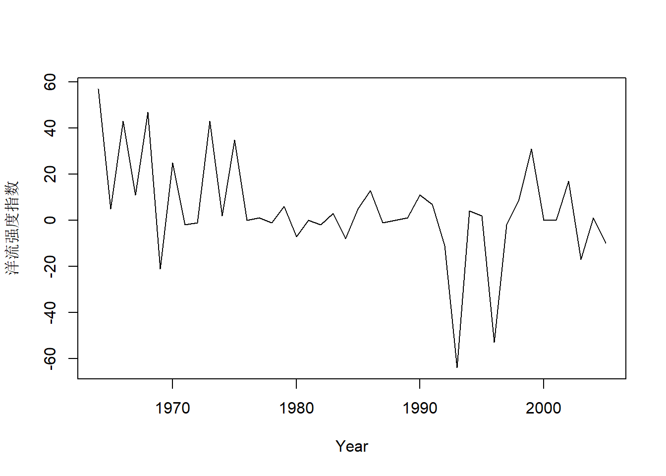
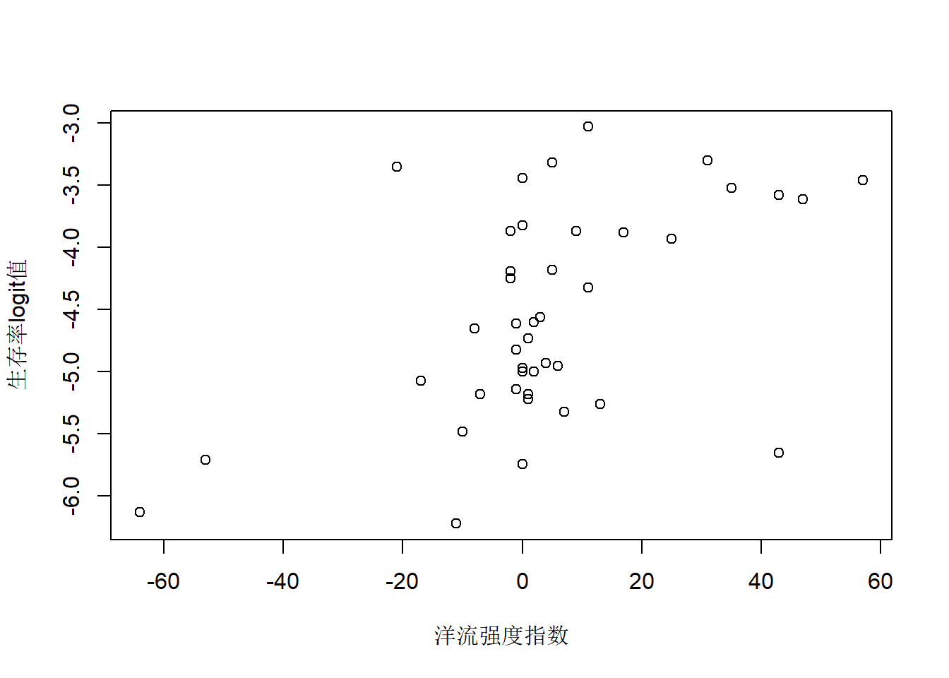
28.5.4 大鳞大马哈鱼生存例子

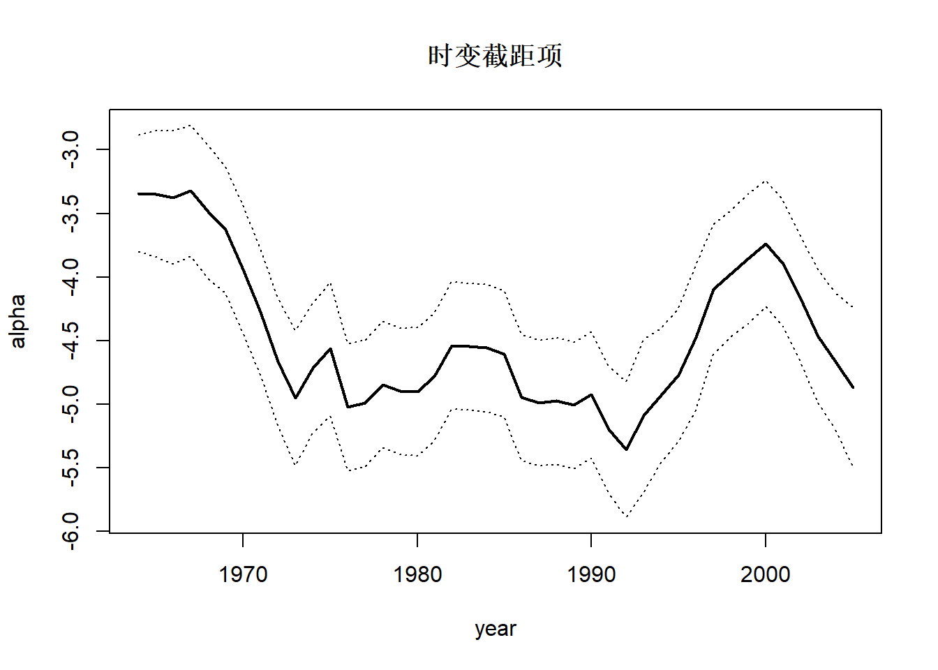
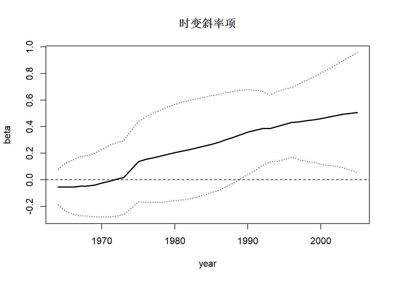
例子来自MARSS手册。研究大鳞大马哈鱼生存状况受到海洋上升洋流强度的影响。海洋上升洋流带来丰富营养，使得近海浮游生物繁盛，有利于大鳞大马哈鱼幼鱼生长。用变系数回归模型： \[ \text{logit(生存率)}_t = \alpha_t + \beta_t \times \text{洋流强度}_t + \nu_t, \ \nu_t \sim \text{N}(0,r) . \] 回归系数模型为 \[ \begin{pmatrix} \alpha_t \\ \beta_t \end{pmatrix} = \begin{pmatrix} 1 & 0 \\ 0 & 1 \end{pmatrix} \begin{pmatrix} \alpha_{t-1} \\ \beta_{t-1} \end{pmatrix} + \boldsymbol w_t, \ \boldsymbol w_t \sim \text{N}(\boldsymbol 0, \text{diag}(q_1, q_2)) . \]

28.5.4.1 数据

library(MARSS)
data(SalmonSurvCUI)
with(SalmonSurvCUI, plot(
  year, logit.s, type="l",
  xlab="Year", ylab="生存率logit值"))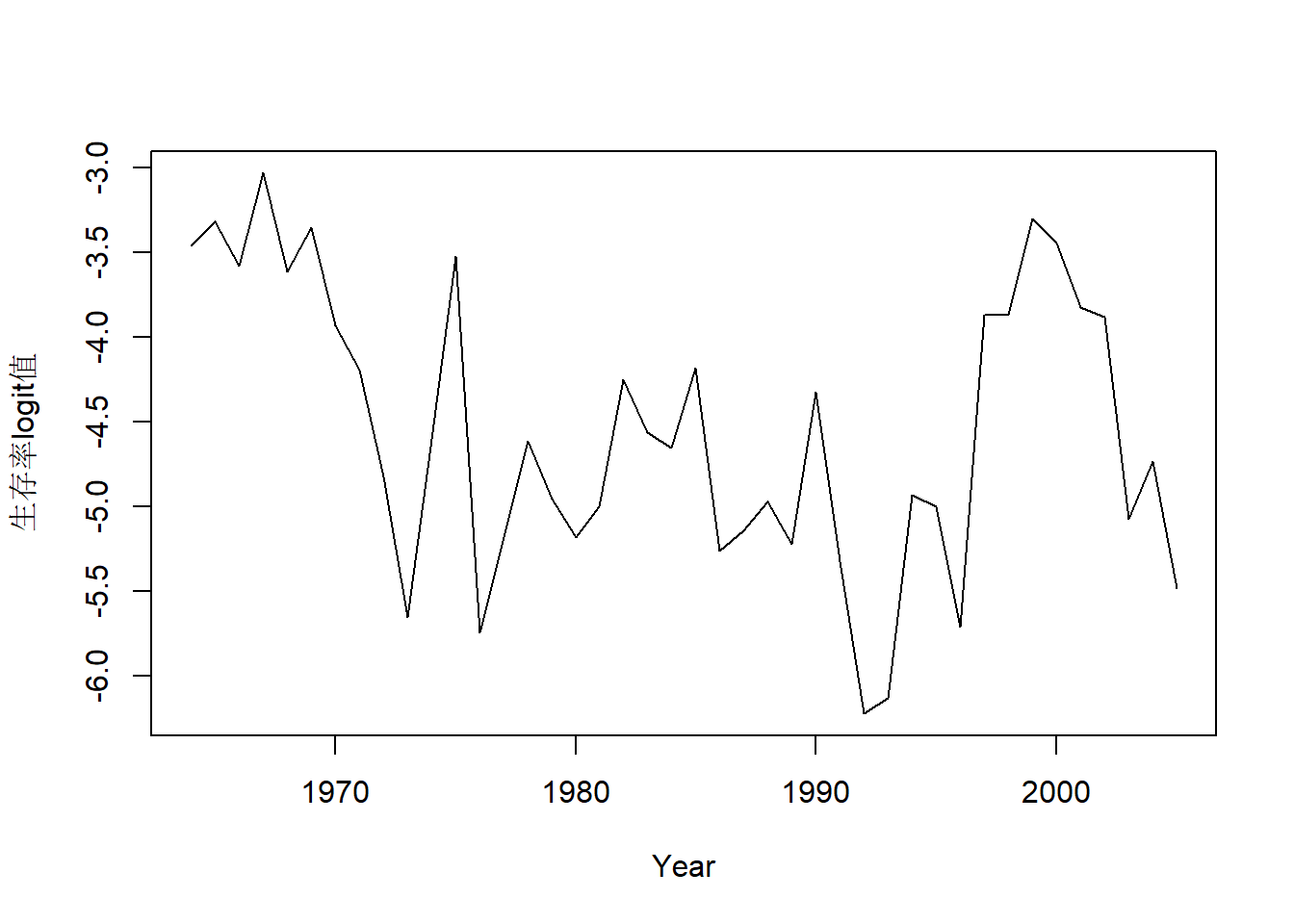

with(SalmonSurvCUI, plot(
  year, CUI.apr, type="l",
  xlab="Year", ylab="洋流强度指数"))

with(SalmonSurvCUI, plot(
  CUI.apr, logit.s, type="p",
  xlab="洋流强度指数", ylab="生存率logit值"))

28.5.4.2 变系数回归建模

# 将输入矩阵的每行作为输出的三维数组的一个子矩阵
# 第三维代表时间$t$
# 适用于一元因变量的多元回归自变量转换为Z矩阵
row2d3 <- function(A){
  A <- t(A)
  dim(A) <- c(1, dim(A))
  A
}

dat <- rbind(SalmonSurvCUI$logit.s)    # 观测变量，回归因变量
CUI.z <- zscore(SalmonSurvCUI$CUI.apr) # 回归自变量，标准化
sal_mod <- list(
  B = "identity",
  U = "zero",
  Q = "diagonal and unequal",
  Z = row2d3(cbind(1, CUI.z)),
  A = "zero",
  R = matrix("r") )
sal_fit1 <- MARSS(
  dat, model = sal_mod,
  inits = list(x0 = cbind(c(0,0))) )

## Success! abstol and log-log tests passed at 115 iterations.
## Alert: conv.test.slope.tol is 0.5.
## Test with smaller values (<0.1) to ensure convergence.
## 
## MARSS fit is
## Estimation method: kem 
## Convergence test: conv.test.slope.tol = 0.5, abstol = 0.001
## Estimation converged in 115 iterations. 
## Log-likelihood: -40.03813 
## AIC: 90.07627   AICc: 91.74293   
##  
##           Estimate
## R.r        0.15708
## Q.(X1,X1)  0.11264
## Q.(X2,X2)  0.00564
## x0.X1     -3.34023
## x0.X2     -0.05388
## Initial states (x0) defined at t=0
## 
## Standard errors have not been calculated. 
## Use MARSSparamCIs to compute CIs and bias estimates.

估计结果为：

\[\begin{aligned} \text{logit(生存率)}_t =& \alpha_t + \beta_t \times \text{洋流强度}_t + \nu_t, \ \nu_t \sim \text{N}(0, 0.16) ; \\ \alpha_t =& \alpha_{t-1} + w_{1t}, \ w_{1t} \sim \text{N}(0, 0.11), \\ \beta_t =& \beta_{t-1} + w_{2t}, \ w_{2t} \sim \text{N}(0, 0.0056) . \end{aligned}\]

提取时变的回归系数：

sal_sm <- tsSmooth(sal_fit1, type="xtT") |>
  pivot_wider(
    id_cols = c("t"),
    names_from = ".rownames",
    values_from = c(".estimate", ".se") ) |>
  mutate(t = t-1 + 1964) |>
  setNames(c("year", "alpha", "beta", "se_alpha", "se_beta")) 
with(sal_sm, {
  ran <- range(c(alpha - 2*se_alpha, alpha + 2*se_alpha))
  plot(year, alpha, type="l", lwd=2, ylim = ran, 
       main="时变截距项")
  lines(year, alpha - 2*se_alpha, lty=3)
  lines(year, alpha + 2*se_alpha, lty=3)
  })

with(sal_sm, {
  ran <- range(c(beta - 2*se_beta, beta + 2*se_beta))
  plot(year, beta, type="l", lwd=2, ylim = ran, 
       main="时变斜率项")
  lines(year, beta - 2*se_beta, lty=3)
  lines(year, beta + 2*se_beta, lty=3)
  abline(h=0, lty=2)
  })

28.5.4.3 预测

应该基于超参数的最大似然估计和\(1:(t-1)\)的观测值来预测时变的回归系数：

sal_pr_co <- tsSmooth(sal_fit1, type = "xtt1")

因变量的预测值，利用\(1:(t-1)\)的信息预测时变回归系数，用\(t\)时刻回归系数预测生存率：

sal_pr <- predict(sal_fit1, type="ytt1")$pred
plot(1964:2005, sal_pr$y, type="b")
lines(1964:2005, sal_pr$estimate, col="red")

残差诊断：

err <- with(sal_pr, y - estimate)
ts.plot(err, main="Residuals", ylab="")
abline(h=0, lty=2)

残差的ACF:

forecast::Acf(err)

残差没有序列自相关。

残差的正态QQ图：

qqnorm(err); qqline(err)

不偏离正态。

28.5.5 时变系数CAPM模型

28.5.5.1 模型

考虑时变系数的资产定价模型(CAPM)： \[\begin{aligned} r_t =& \beta_{0t} + \beta_{1t} r_{M,t} + e_t, \ e_t \sim \text{ iid N}(0, \sigma_e^2), \\ \beta_{0,t+1} =& \beta_{0,t} + u_t, \ u_t \sim \text{ iid N}(0, \sigma_{u}^2), \\ \beta_{1,t+1} =& \beta_{1,t} + v_t, \ v_t \sim \text{ iid N}(0, \sigma_{v}^2), \end{aligned}\] 其中\(\{e_t\}\), \(\{u_t\}\), \(\{v_t\}\)相互独立， \(r_t\)是某金融资产的超额收益率， \(r_{M,t}\)是市场的超额收益率。可以写成状态空间模型 \[\begin{aligned} r_t =& (1, r_{M,t}) \begin{pmatrix} \beta_{0t} \\ \beta_{1t} \end{pmatrix} + e_t, \\ \begin{pmatrix} \beta_{0,t+1} \\ \beta_{1,t+1} \end{pmatrix} =& \begin{pmatrix} 1 & 0 \\ 0 & 1 \end{pmatrix} \begin{pmatrix} \beta_{0,t} \\ \beta_{1,t} \end{pmatrix} + \begin{pmatrix} u_t \\ v_t \end{pmatrix} . \end{aligned}\] 令状态变量\(\boldsymbol \alpha_t = (\beta_{0t}, \beta_{1t})^T\), 观测变量为\(r_t\)，且 \[\begin{aligned} Z_t =& (1, r_{M,t}) , \quad H_t = \sigma_e^2, \\ T_t =& I_2, \quad R_t = I, \quad \boldsymbol\eta_t = (u_t, v_t)^T, \\ Q_t =& \begin{pmatrix} \sigma_u^2 & 0 \\ 0 & \sigma_v^2 \end{pmatrix} , \end{aligned}\] 则时变系数CAPM对应于状态空间模型 \[\begin{aligned} r_t =& Z_t \boldsymbol\alpha_t + e_t, \ e_t \sim \text{N}(0, H_t), \\ \boldsymbol\alpha_{t+1} =& T_t \boldsymbol\alpha_t + R_t \boldsymbol\eta_t, \ \boldsymbol\eta_t \sim \text{N}(0, Q_t) . \end{aligned}\]

28.5.5.2 通用动力的例子

例28.8 考虑通用动力(GM)股票的月度超额收益率\(r_t\)的CAPM模型，时间为1990年1月到2003年12月，以标普500超额收益率为市场超额收益率\(r_{M,t}\)。

数据（收益率单位：百分之一）：

da_gm <- readr::read_table(
  "m-fac9003.txt",
  col_types = cols(.default=col_double()))[,c("GM", "SP5")]
nda <- nrow(da_gm)
ts.gm <- ts(as.matrix(da_gm),
  start=c(1990, 1), frequency=12)
plot(as.xts(ts.gm),
  main="GM和标普500的月度超额收益率(%)")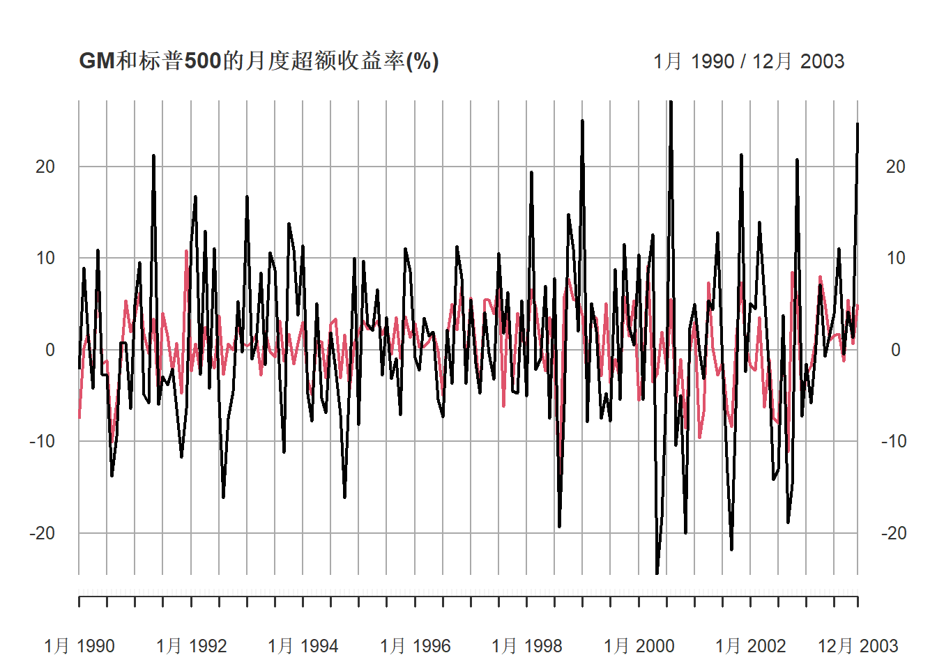

28.5.5.3 滚动计算回归的简单做法

尝试滚动地进行线性回归，取固定的拟合时间窗口为24个月，获得动态的系数估计：

wh <- 24 # 滚动窗口
n <- nrow(da_gm)
betamat <- matrix(NA, n, 2)
for(t in wh:n){
  tind <- (t-wh+1):t
  betamat[t,] <- 
    lm(GM ~ SP5, data=da_gm[tind,]) |>
    coef()
}
plot(ts(
  betamat[,1], 
  start=c(1990, 1), 
  frequency=12),
  main="Time varying intercept",
  ylab="")

plot(ts(
  betamat[,2], 
  start=c(1990, 1), 
  frequency=12),
  main="Time varying slope",
  ylab="")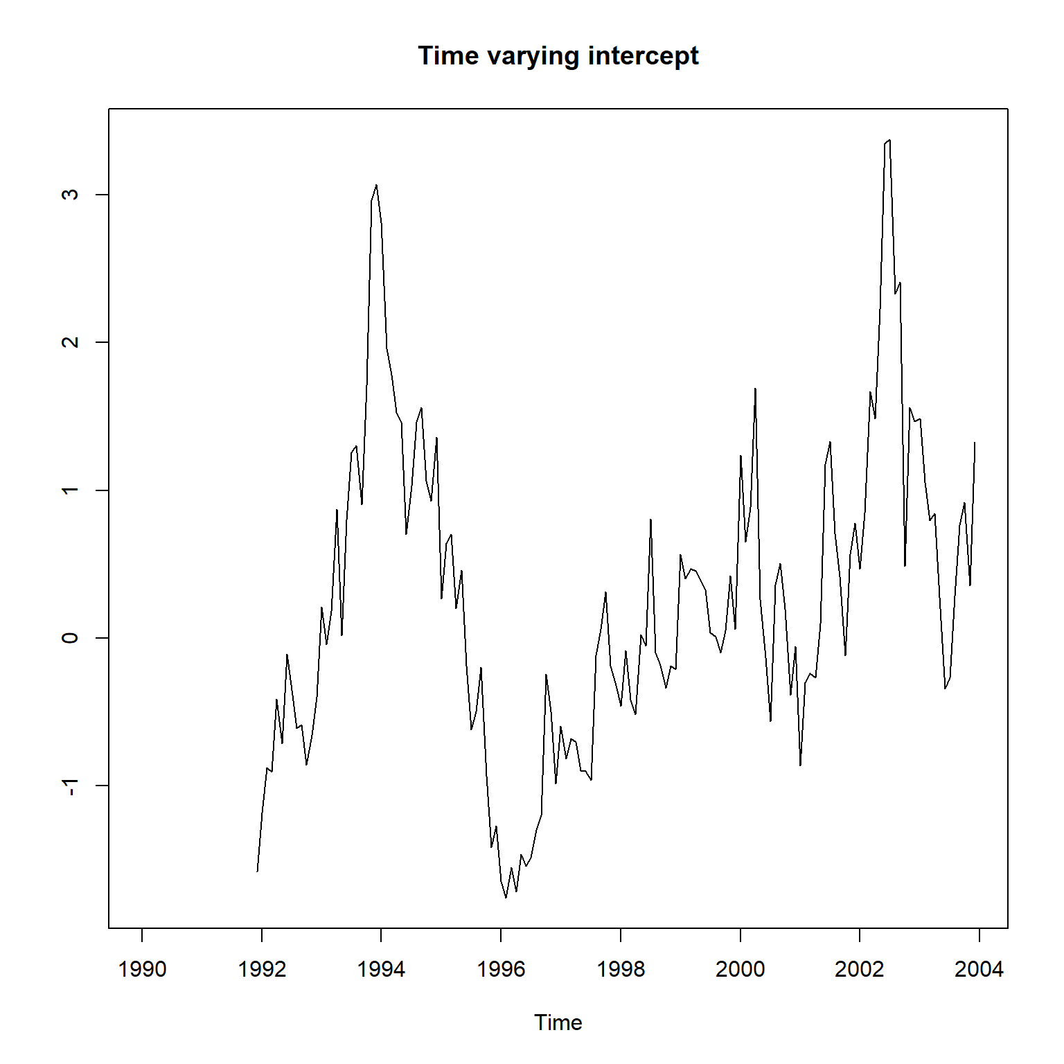

这个结果可以作为基准。

28.5.5.4 使用KFAS包拟合时变系数回归模型

statespacer包没有提供时变系数回归模型，而\(Z_t\)依赖于\(t\)时statespacer包没有提供自定义方法。

使用KFAS包。这个包提供了SSMregression()函数，可以指定带有随机游动斜率的回归模型，但不支持随机截距项，尝试使用自定义的对应于截距项的自变量会使得滤波平滑失败。

我们使用SScustom()直接指定各个矩阵。 KFAS对时变的\(Z_t\)等模型矩阵，允许直接输入一个三维数组Z， Z[,,t]的值为\(Z_t\)。

\(Z_t\), \(T_t\), \(H_t\), \(Q_t\)等矩阵如果输入为三维矩阵，就是时变的；如果输入为二维矩阵，就是非时变的，也可以输入为标量，就相当于非时变的\(1\times 1\)矩阵。

library(KFAS)

# 将每一行是一个$Z_t$值的矩阵，
# 转换成$1 \times m \times n$的数组，
# $m$是状态空间维数，$n$是样本量
dim2to3 <- function(M){
  M <- t(M)
  dim(M) <- c(1, dim(M))
  M
}

# Zt: 用三维数组表示的$Z_t, t=1,2,\dots,n$，
# 第三下标代表$t$,
# Zt[,,t]是$1 \times m$矩阵$Z_t$
Zt <- dim2to3(cbind(1, da_gm[["SP5"]]))

mod_gm <- SSModel(
  da_gm$GM ~ SSMcustom(
    Z = Zt, # 观测方程的载荷阵
    T = diag(2), # 状态方程的转移矩阵
    # 状态的初始值
    a1 = c(0, 1),
    # Q是状态方程扰动项方差阵
    Q = diag(NA, 2)),
  # H是观测方程误差方差阵
  H = NA)
fit_gm <- fitSSM(
  mod_gm, 
  inits = c(0,0,0), 
  method="BFGS") #"Nelder-Mead") 
fit_gm$optim.out$value

## [1] 589.0349

估计的随机截距和随机斜率的扰动标准差：

sqrt(diag(fit_gm$model$Q[,,1]))

## [1] 0.0043620203 0.0006551979

这两个标准差接近于0，说明估计的时变截距项和时变斜率项近似等于常数值。

估计的回归误差项标准差：

sqrt(fit_gm$model$H[,,1])

## [1] 8.108269

计算平滑结果：

res_gm <- KFS(fit_gm$model)

GM原始值与拟合值（使用平滑）的曲线：

plot(ts.gm[,"GM"], main="GM and fitted")
lines(as.vector(time(ts.gm)), 
  c(fitted(res_gm, filtered=FALSE)),
  col="red")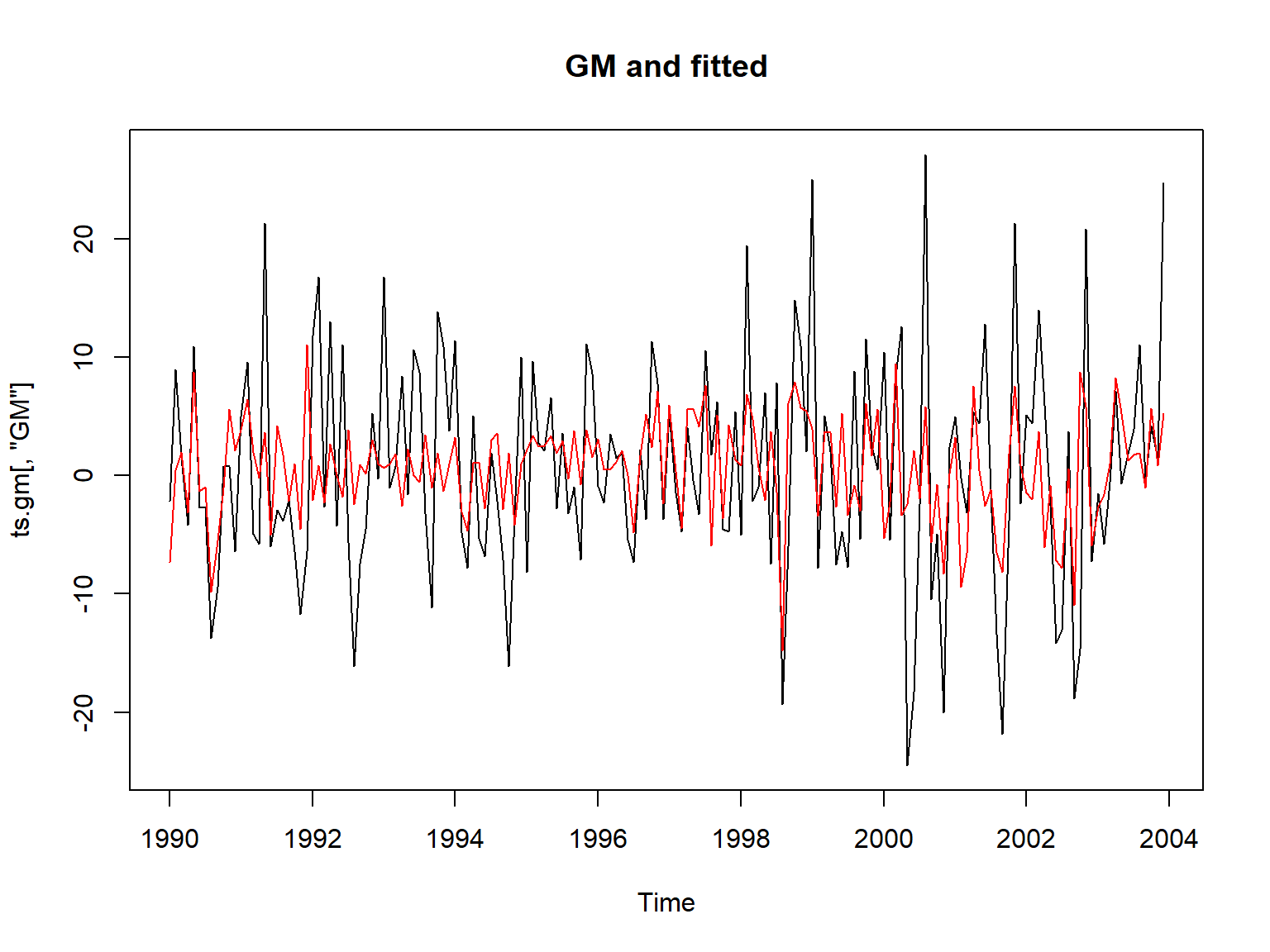

如果前面的程序中没有指定a1 = c(0, 1)，即初始的随机截距、随机斜率，则拟合上图在左端的拟合效果很差。

估计的时变截距项和时变斜率项：

states <- as.matrix(coef(res_gm))
states[,2] <- states[,1] + states[,2]
states <- states[,2:3]
plot(ts(states[,1], start=c(1990, 1), frequency=12),
  main = "Time-varying intercept",
  ylab = "",
  ylim = c(-0.5, 0.5))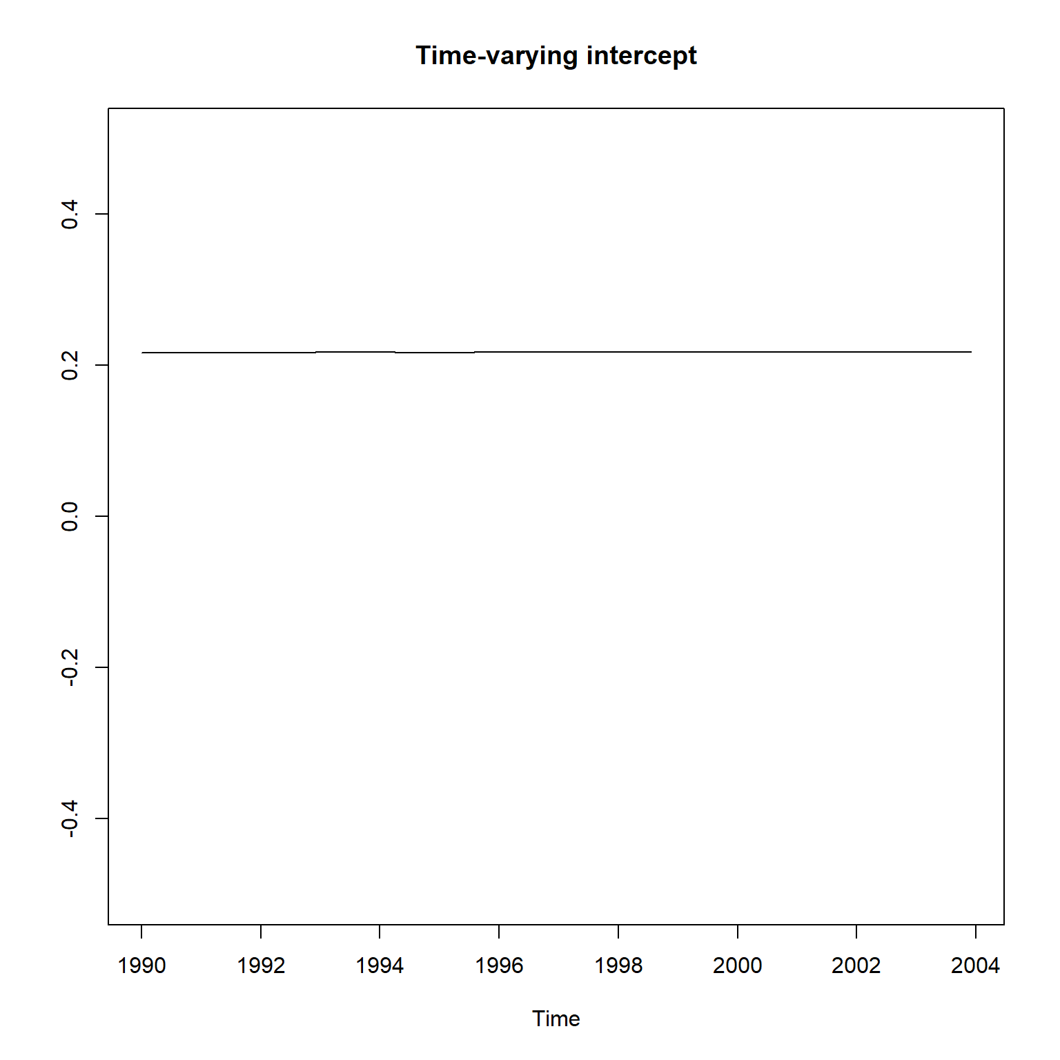

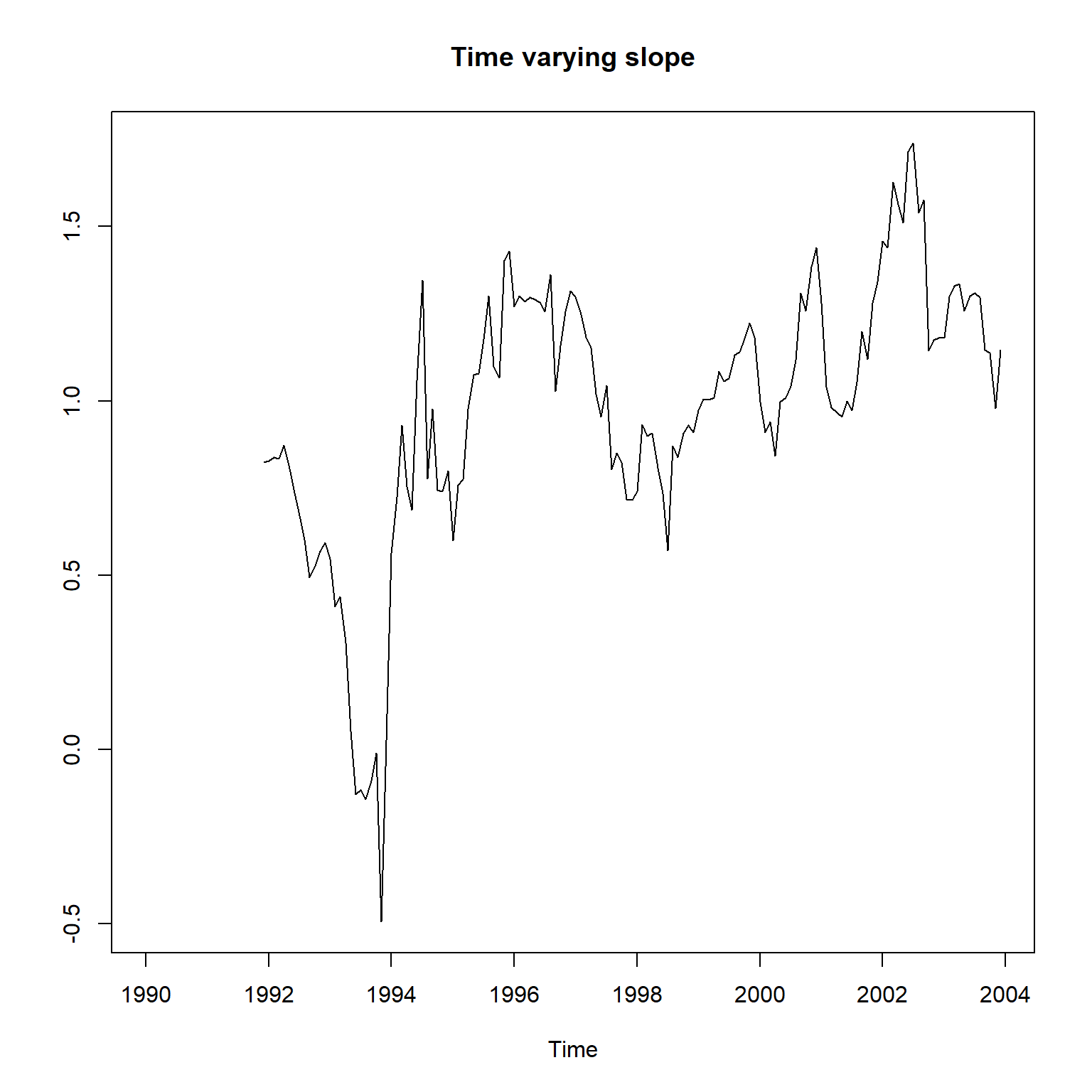
plot(ts(states[,2], start=c(1990, 1), frequency=12),
  main = "Time-varying slope",
  ylab="", 
  ylim = c(0, 1.5))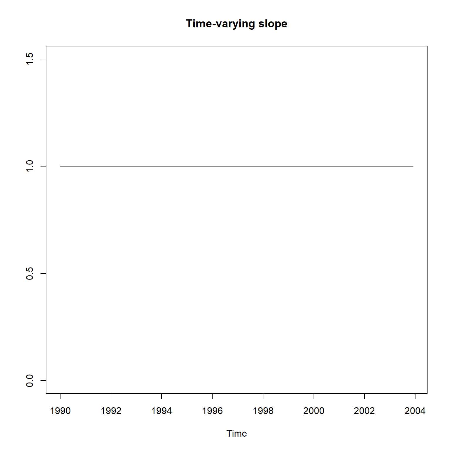

可以看出，时变的截距项\(\beta_{0t}\)和时变斜率项\(\beta_{1t}\)基本上取常数值，与滚动回归得到的结果不一致，没有起到时变的效果。

使用KFAS的SSMregression()，仅使用随机斜率项：

mod_gm <- SSModel(
  da_gm$GM ~ SSMregression(
    ~ da_gm$SP5,
    # Q是状态方程扰动项方差阵
    Q = NA),
  # H是观测方程误差方差阵
  H = NA)
fit_gm <- fitSSM(
  mod_gm, 
  inits = c(0, 0), 
  method="BFGS")
res_gm <- KFS(fit_gm$model)

拟合结果：

plot(ts.gm[,"GM"], main="GM and fitted with time-varying beta")
lines(as.vector(time(ts.gm)), 
  c(fitted(res_gm, filtered=FALSE)),
  col="red")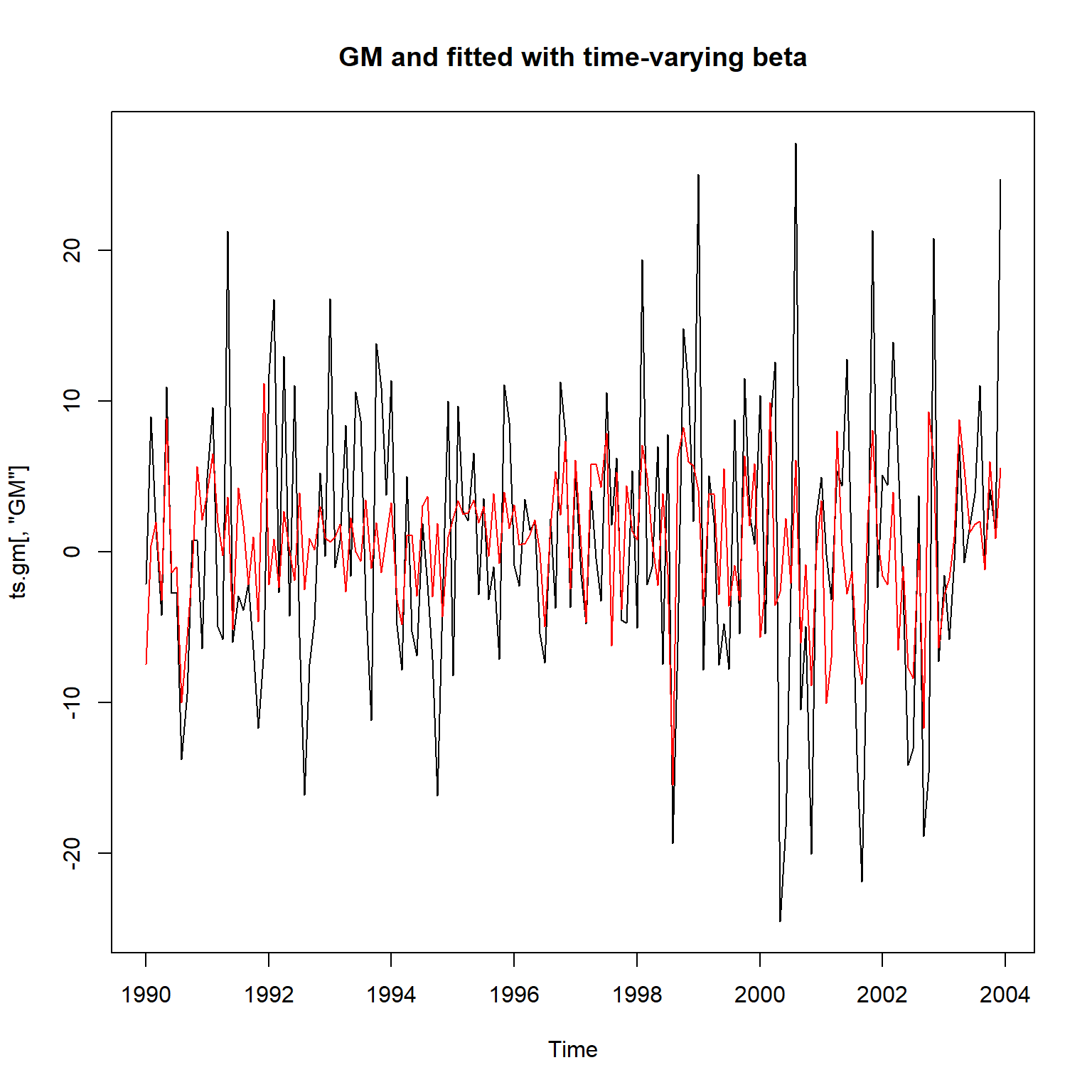

这个拟合结果比较合理。

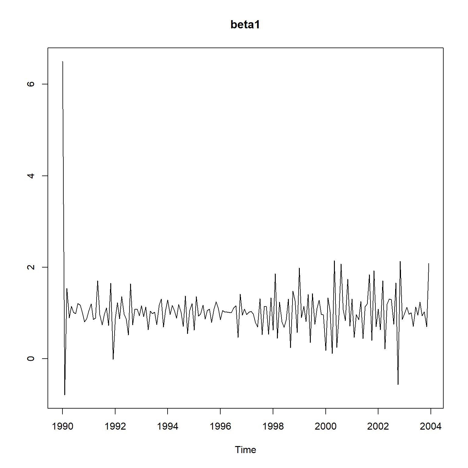
随机斜率项估计：

states <- as.matrix(coef(res_gm))
plot(ts(states[,2], start=c(1990, 1), frequency=12),
  main="Time-varying Regression Slope",
  ylab="",
  ylim = c(0.5, 1.5))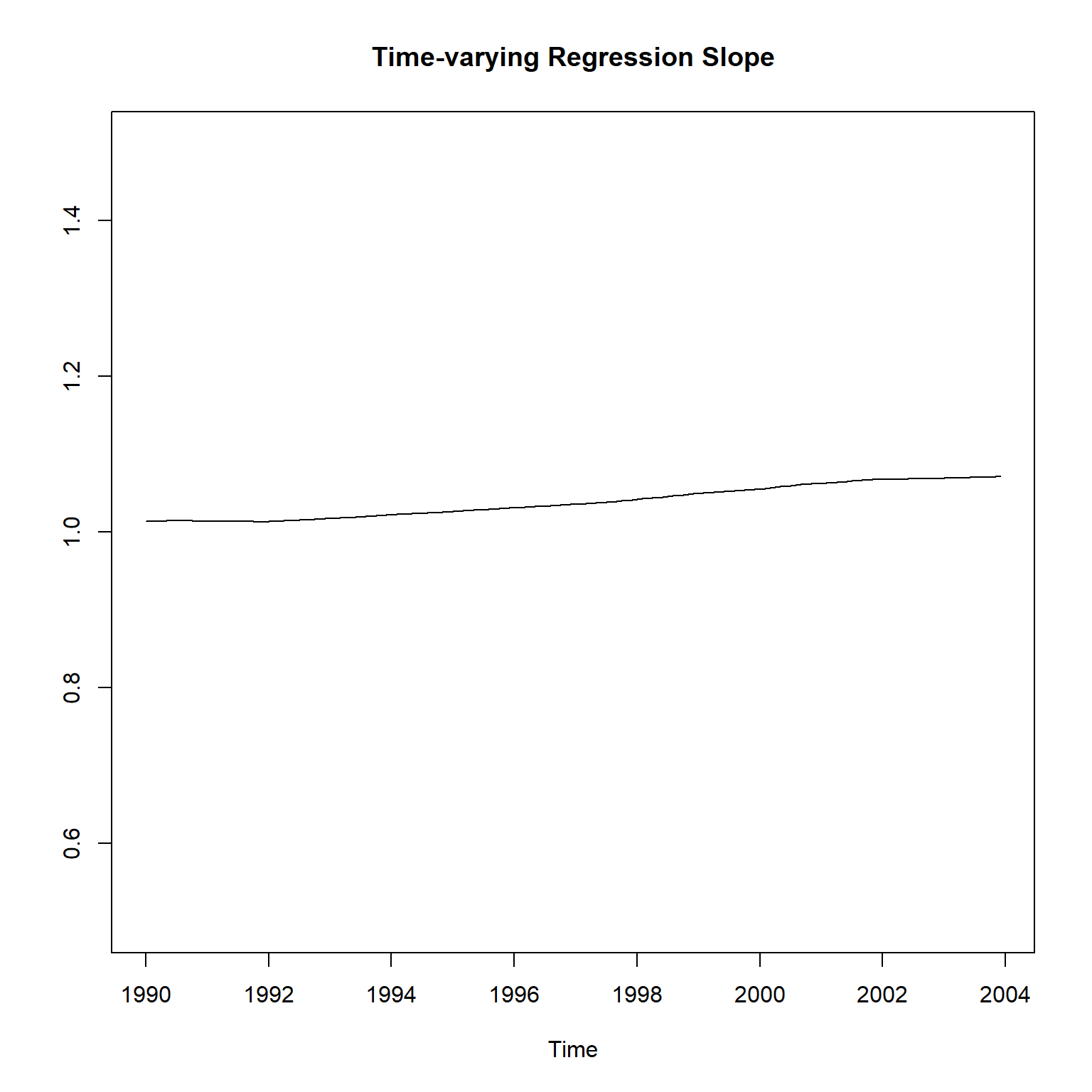

这个结果与滚动窗口回归计算的斜率项还是不一致，但是变化范围比较小，有一定合理性。

28.5.5.5 使用dlm包拟合时变系数回归模型

dlm包也支持时变系数回归，可以用dlm尝试估计时变截距和斜率。

输入超参数的建模函数：

library(dlm)
buildFun <- function(para){
  dlmModReg(
    cbind(da_gm[["SP5"]]), # 自变量值
    dV = exp(para[1]),  # 回归误差方差
    dW= exp(para[2:3])) # 状态方程误差方差
}

超参数最大似然估计：

fit_dlm <- dlmMLE(
  da_gm[["GM"]],
  parm = c(0,-2,-2),
  build = buildFun)
fit_dlm$conv

## [1] 0

估计的数值算法收敛。提取最优参数的模型：

dlm_gm <- buildFun(fit_dlm$par)

回归误差项标准差：

V(dlm_gm) |> sqrt()

##          [,1]
## [1,] 8.130086

随机截距项和斜率项的标准差：

W(dlm_gm) |> diag() |> sqrt()

## [1] 9.177050e-04 1.271935e-06

估计得到的状态方程扰动项标准差很小，比KFAS模型得到的结果小得多，使得截距和斜率基本等于常数。

利用最大似然估计得到的超参数进行滤波和平滑：

filt_gm <- dlmFilter(da_gm[["GM"]], dlm_gm)
smth_gm <- dlmSmooth(filt_gm)

平滑得到的时变截距项和时变斜率项：

plot(ts(
  smth_gm$s[-1,1], 
  start=c(1990, 1), 
  frequency=12),
  ylim=c(0,1),
  main="Time-varying intercept",
  ylab="")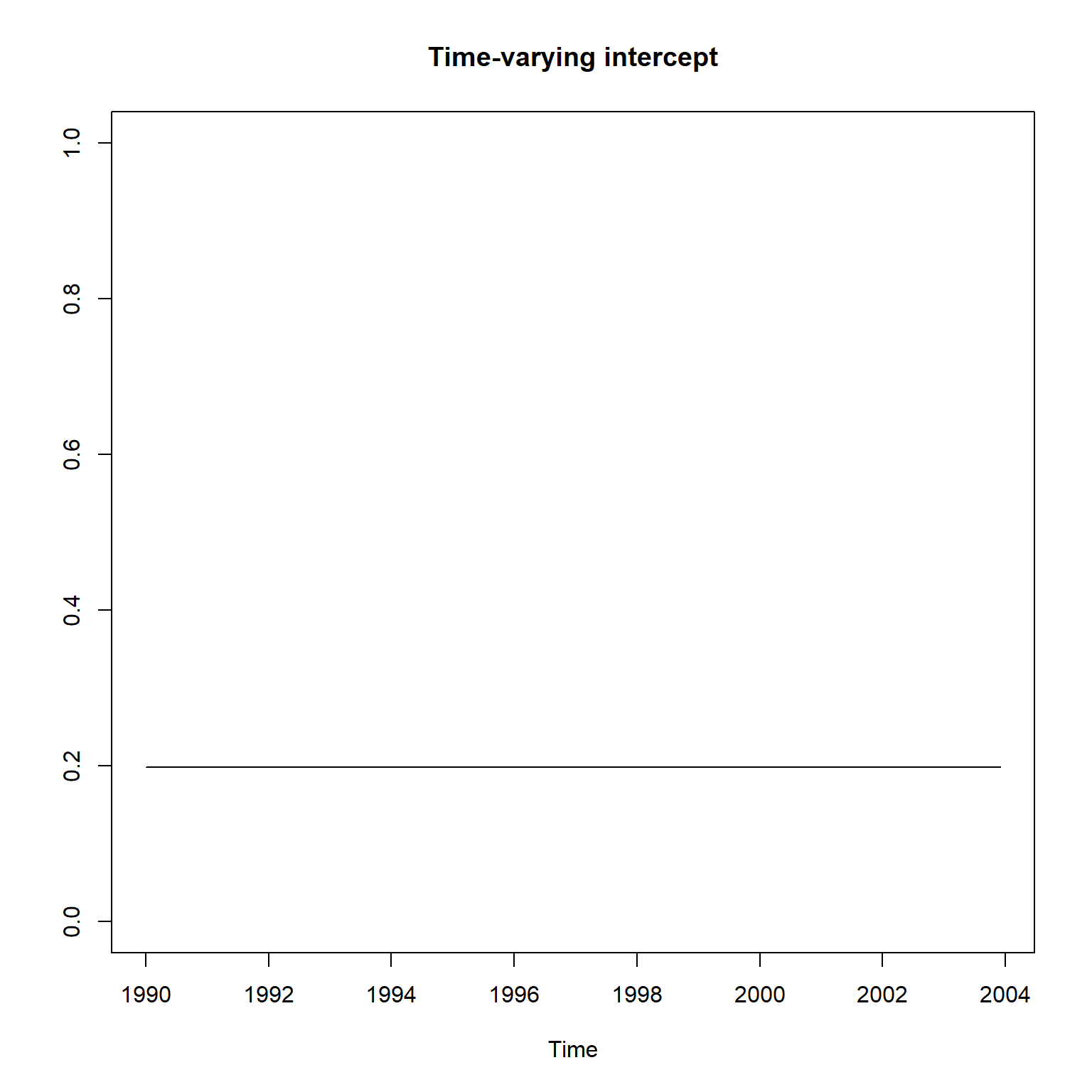

plot(ts(
  smth_gm$s[-1,2], 
  start=c(1990, 1), 
  frequency=12),
  ylim=c(0.5, 1.5),
  main="Time-varying slope",
  ylab="")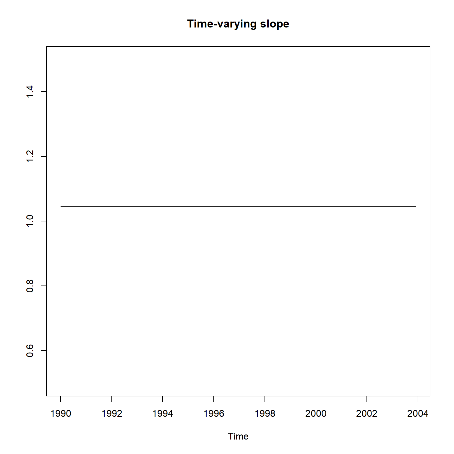

与KFAS的结果不一致。另外，实际上截距和斜率的变化范围很小，基本上是常数。

28.5.5.6 使用MARSS包拟合时变系数回归模型

library(MARSS)

mod_capm <- list(
    B = "identity",
    U = "zero",
    Q = "diagonal and unequal",
    Z = row2d3(cbind(1, da_gm$SP5)),
    A = "zero",
    R = matrix("r"),
    x0 = cbind(c("b00", "b10"))  )
fit_capm_em <- MARSS(
  rbind(da_gm$GM),
  model = mod_capm,
  control = list(maxit=100), 
  inits = list(x0 = cbind(c(0,0))) )

## Warning! Reached maxit before parameters converged. Maxit was 100.
##  neither abstol nor log-log convergence tests were passed.
## 
## MARSS fit is
## Estimation method: kem 
## Convergence test: conv.test.slope.tol = 0.5, abstol = 0.001
## WARNING: maxit reached at  100  iter before convergence.
##  Neither abstol nor log-log convergence test were passed.
##  The likelihood and params are not at the MLE values.
##  Try setting control$maxit higher.
## Log-likelihood: -596.9282 
## AIC: 1203.856   AICc: 1204.227   
##  
##           Estimate
## R.r        65.7133
## Q.(X1,X1)   0.1995
## Q.(X2,X2)   0.0254
## x0.b00      0.2843
## x0.b10      0.9198
## Initial states (x0) defined at t=0
## 
## Standard errors have not been calculated. 
## Use MARSSparamCIs to compute CIs and bias estimates.
## 
## Convergence warnings
##  Warning: the  Q.(X1,X1)  parameter value has not converged.
##  Warning: the  Q.(X2,X2)  parameter value has not converged.
##  Warning: the  x0.b00  parameter value has not converged.
##  Warning: the  logLik  parameter value has not converged.
##  Type MARSSinfo("convergence") for more info on this warning.

fit_capm <- MARSS(
  rbind(da_gm$GM),
  model = mod_capm,
  inits = fit_capm_em$par, 
  method = "BFGS")

## Success! Converged in 11 iterations.
## Function MARSSkfas used for likelihood calculation.
## 
## MARSS fit is
## Estimation method: BFGS 
## Estimation converged in 11 iterations. 
## Log-likelihood: -589.4323 
## AIC: 1188.865   AICc: 1189.235   
##  
##           Estimate
## R.r       6.53e+01
## Q.(X1,X1) 1.07e-10
## Q.(X2,X2) 3.01e-13
## x0.b00    1.98e-01
## x0.b10    1.05e+00
## Initial states (x0) defined at t=0
## 
## Standard errors have not been calculated. 
## Use MARSSparamCIs to compute CIs and bias estimates.

提取\(\beta_{0t}\)和\(\beta_{1t}\)的估计序列：

extract_tvc <- function(mfit){
  res <- tsSmooth(mfit, type="xtT")
  sm <- ts(
    cbind(res[res$.rownames=="X1", ".estimate"],
          res[res$.rownames=="X2", ".estimate"]),
    start=c(1990, 1), frequency=12)
  sm
}
sm <- extract_tvc(fit_capm)
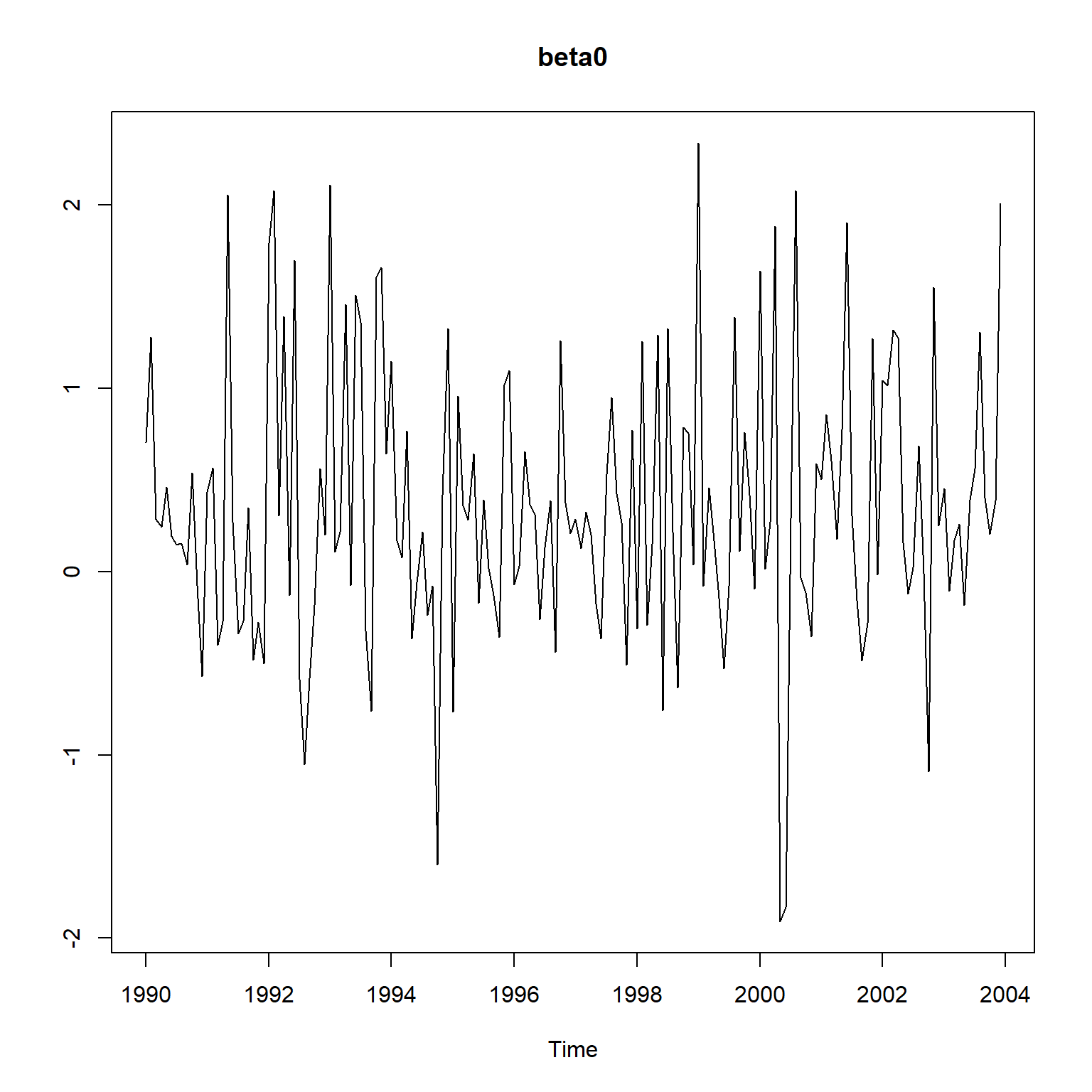
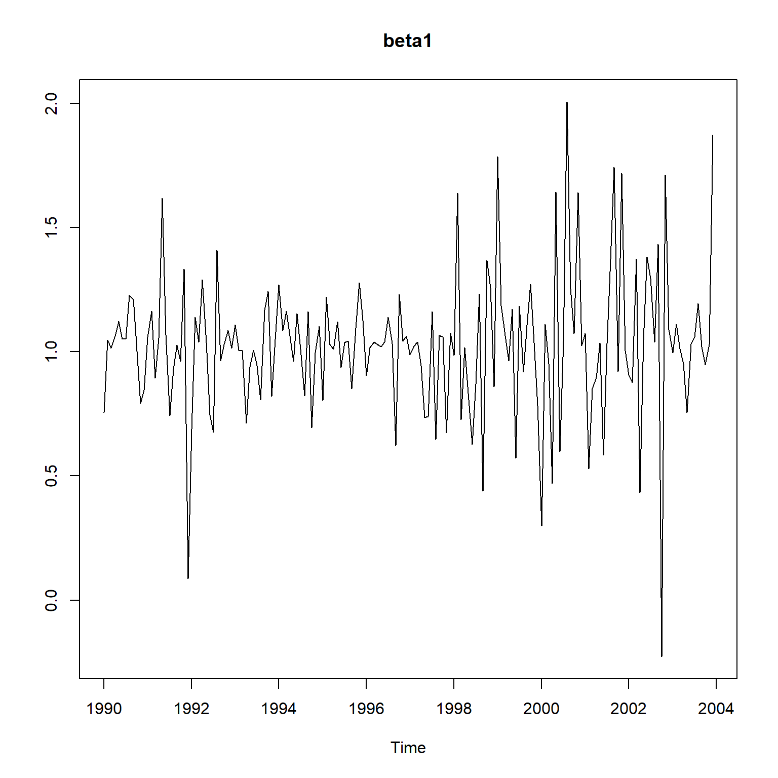
plot(sm[,1], ylim=c(0,1), main="beta0", ylab="")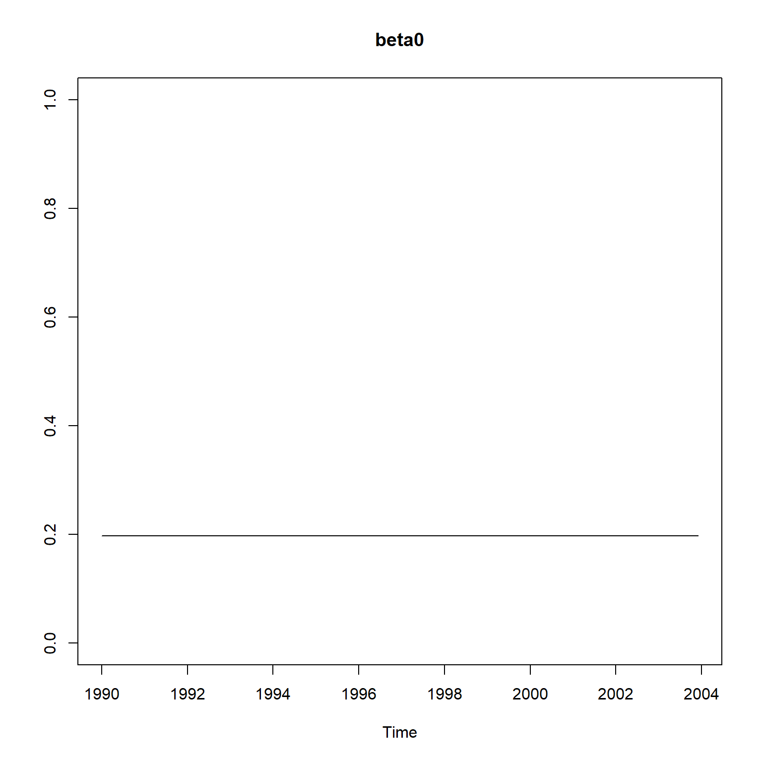

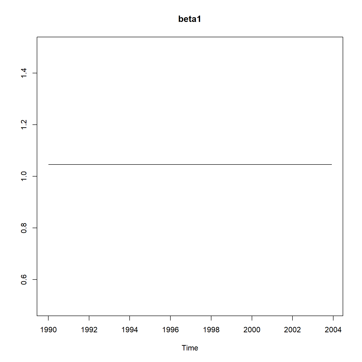
plot(sm[,2], ylim=c(0.5,1.5), main="beta1", ylab="")

结果与KFAS, dlm包结果类似，都相当于非时变的情形。

序列拟合结果：

res_capm_y <- fitted(fit_capm, type="ytT")
plot(ts.gm[,1], main="GM and fitted")
lines(as.vector(time(ts.gm)), res_capm_y$.fitted, col="red")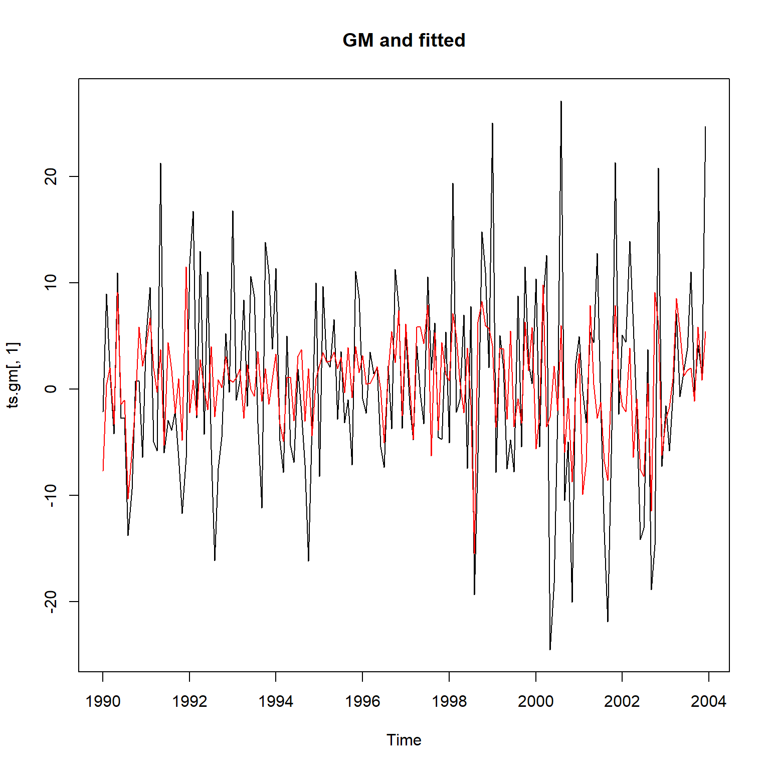

28.5.5.7 模型改进

前面的状态空间模型中时变的回归系数用了随机游动，注意随机游动是非平稳时间序列模型。计算结果都接近于常系数结果。

下面用平稳的VAR(1)模型作为回归系数模型。设 \[\begin{aligned} r_t =& \beta_{0t} + \beta_{1t} r_{M,t} + e_t, \ e_t \sim \text{ iid N}(0, \sigma_e^2), \\ \beta_{0,t+1} =& b_{00} + b_{01} \beta_{0,t} + u_t, \ u_t \sim \text{ iid N}(0, \sigma_{u}^2), \\ \beta_{1,t+1} =& b_{10} + b_{11} \beta_{1,t} + v_t, \ v_t \sim \text{ iid N}(0, \sigma_{v}^2) . \end{aligned}\]

mod_capm2 <- list(
    B = "diagonal and unequal",
    U = "unconstrained",
    Q = "diagonal and unequal",
    Z = row2d3(cbind(1, da_gm$SP5)),
    A = "zero",
    R = matrix("r"),
    x0 = cbind(c(mean(da_gm$GM), 0)),
    V0 = diag(1E6, 2))
fit_capm_em2 <- MARSS(
  rbind(da_gm$GM),
  model = mod_capm2,
  control = list(maxit=100))

## Warning! Reached maxit before parameters converged. Maxit was 100.
##  neither abstol nor log-log convergence tests were passed.
## 
## MARSS fit is
## Estimation method: kem 
## Convergence test: conv.test.slope.tol = 0.5, abstol = 0.001
## WARNING: maxit reached at  100  iter before convergence.
##  Neither abstol nor log-log convergence test were passed.
##  The likelihood and params are not at the MLE values.
##  Try setting control$maxit higher.
## Log-likelihood: -588.658 
## AIC: 1191.316   AICc: 1192.016   
##  
##           Estimate
## R.r       47.40402
## B.(X1,X1)  0.01852
## B.(X2,X2) -0.00013
## U.X1       0.32866
## U.X2       1.03591
## Q.(X1,X1)  5.90385
## Q.(X2,X2)  0.70689
## Initial states (x0) defined at t=0
## 
## Standard errors have not been calculated. 
## Use MARSSparamCIs to compute CIs and bias estimates.
## 
## Convergence warnings
##  Warning: the  logLik  parameter value has not converged.
##  Type MARSSinfo("convergence") for more info on this warning.

fit_capm2 <- MARSS(
  rbind(da_gm$GM),
  model = mod_capm2,
  inits = fit_capm_em2$par, 
  method = "BFGS")

## Success! Converged in 11 iterations.
## Function MARSSkfas used for likelihood calculation.
## 
## MARSS fit is
## Estimation method: BFGS 
## Estimation converged in 11 iterations. 
## Log-likelihood: -587.9871 
## AIC: 1189.974   AICc: 1190.674   
##  
##            Estimate
## R.r        4.83e+01
## B.(X1,X1) -2.78e-05
## B.(X2,X2) -9.40e-06
## U.X1       3.51e-01
## U.X2       1.03e+00
## Q.(X1,X1)  5.99e+00
## Q.(X2,X2)  6.12e-01
## Initial states (x0) defined at t=0
## 
## Standard errors have not been calculated. 
## Use MARSSparamCIs to compute CIs and bias estimates.

用了扩散先验。但是，平稳的VAR(1)模型需要其初始值分布服从平稳分布，否则会影响系数矩阵\(B\)的估计。结果的时变回归系数基本是白噪声。改进效果不好。时变回归系数估计结果图形：

sm <- extract_tvc(fit_capm2)
plot(sm[,1], main="beta0", ylab="")

plot(sm[,2], main="beta1", ylab="")

将初始时间点设为\(t=1\)：

mod_capm3 <- list(
    B = "diagonal and unequal",
    U = "unconstrained",
    Q = "diagonal and unequal",
    Z = row2d3(cbind(1, da_gm$SP5)),
    A = "zero",
    R = matrix("r"),
    tinitx = 1
    )
fit_capm_em3 <- MARSS(
  rbind(da_gm$GM),
  model = mod_capm3,
  inits = list(x0 = cbind(c(0,0))),
  control = list(maxit=100))

## Warning! Reached maxit before parameters converged. Maxit was 100.
##  neither abstol nor log-log convergence tests were passed.
## 
## MARSS fit is
## Estimation method: kem 
## Convergence test: conv.test.slope.tol = 0.5, abstol = 0.001
## WARNING: maxit reached at  100  iter before convergence.
##  Neither abstol nor log-log convergence test were passed.
##  The likelihood and params are not at the MLE values.
##  Try setting control$maxit higher.
## Log-likelihood: -586.2302 
## AIC: 1190.46   AICc: 1191.6   
##  
##           Estimate
## R.r         44.938
## B.(X1,X1)    0.159
## B.(X2,X2)   -0.314
## U.X1         0.235
## U.X2         1.329
## Q.(X1,X1)    5.189
## Q.(X2,X2)    0.778
## x0.X1       46.751
## x0.X2        6.486
## Initial states (x0) defined at t=1
## 
## Standard errors have not been calculated. 
## Use MARSSparamCIs to compute CIs and bias estimates.
## 
## Convergence warnings
##  Warning: the  x0.X1  parameter value has not converged.
##  Warning: the  x0.X2  parameter value has not converged.
##  Type MARSSinfo("convergence") for more info on this warning.

fit_capm3 <- MARSS(
  rbind(da_gm$GM),
  model = mod_capm3,
  inits = fit_capm_em3$par, 
  method = "BFGS")

## Success! Converged in 17 iterations.
## Function MARSSkfas used for likelihood calculation.
## 
## MARSS fit is
## Estimation method: BFGS 
## Estimation converged in 17 iterations. 
## Log-likelihood: -586.164 
## AIC: 1190.328   AICc: 1191.467   
##  
##            Estimate
## R.r        5.10e+01
## B.(X1,X1)  1.68e-01
## B.(X2,X2) -3.35e-01
## U.X1       2.21e-01
## U.X2       1.36e+00
## Q.(X1,X1)  1.83e-06
## Q.(X2,X2)  6.96e-01
## x0.X1      4.69e+01
## x0.X2      6.50e+00
## Initial states (x0) defined at t=1
## 
## Standard errors have not been calculated. 
## Use MARSSparamCIs to compute CIs and bias estimates.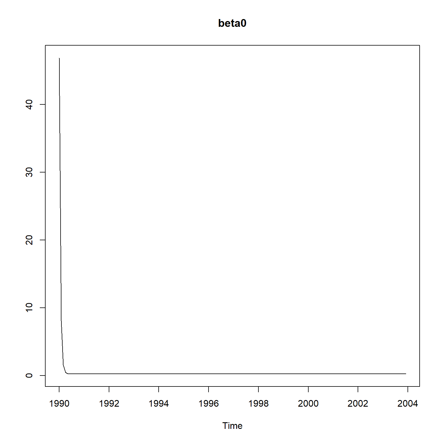

sm <- extract_tvc(fit_capm3)
plot(sm[,1], main="beta0", ylab="")

plot(sm[,2], main="beta1", ylab="")

初值估计还是有较大问题。

28.5.6 带有ARMA误差的回归模型

设 \[\begin{aligned} y_t = \boldsymbol X_t \boldsymbol\beta + \xi_t, \end{aligned}\] \(\xi_t\)服从ARMA模型，可以写成状态空间形式，状态方程为 \[ \boldsymbol\alpha_{t+1} = T \boldsymbol\alpha_t + R \boldsymbol\eta_t, \] 则\(y_t\)可以写成状态空间模型形式，状态变量为\(\boldsymbol\alpha_t^*\)，模型为 \[\begin{aligned} \boldsymbol\alpha_t^* =& \begin{pmatrix} \boldsymbol\beta \\ \boldsymbol\alpha_t \end{pmatrix}, \\ y_t =& (\boldsymbol X_t, 1, 0, \dots, 0) \boldsymbol\alpha_t^*, \\ \boldsymbol\alpha_{t+1}^* =& \begin{pmatrix} I_k & 0 \\ 0 & T \end{pmatrix} \boldsymbol\alpha_t^* + \begin{pmatrix} 0 \\ R \end{pmatrix} \eta_t, \end{aligned}\] 可以用状态空间模型的工具进行估计和推断。

MARSS包直接支持协变量回归，所以可以将时变误差放在系统方程中，将协变量回归放在观测方程中，观测方程中还可以带有本身的独立观测误差： \[\begin{aligned} x_t =& b x_{t-1} + w_t, \ w_t \sim \text{N}(0,q), \\ y_t =& x_t + \alpha + (\beta_1, \beta_2, \dots) (d_{1t}, d_{2t}, \dots)^T + v_t, \ v_t \sim \text{N}(0, r) . \end{aligned}\]

28.5.7 动态Nelson-Siegel模型

考虑如下的关于利率期限结构的动态Nelson-Siegel模型： \[\begin{aligned} y_t(\tau) =& \beta_{1t} + \beta_{2t} \left( \frac{1 - e^{-\lambda \tau}}{\lambda \tau} \right) + \beta_{3t} \left( \frac{1 - e^{-\lambda \tau}}{\lambda \tau} - e^{-\lambda \tau} \right) + e_t(\tau), \\ & \tau=3, 6, 12, 24, 36, 60, 84, 120, \ t=1,2,\dots, n . \end{aligned}\] 其中\(\lambda\)是未知参数， \(\tau\)是贷款期限， \(y_t(\tau)\)是\(t\)时刻期限为\(\tau\)的贷款利息。设各\(e_t(\tau)\)相互独立，服从\(\text{N}(0, \sigma_e^2)\)； \(\beta_{1t}\), \(\beta_{2t}\), \(\beta_{3t}\)是时变的回归系数，设其服从一阶向量自回归模型： \[ \boldsymbol\beta_{t+1} =(I - \Phi) \boldsymbol\mu + \Phi\boldsymbol\beta_t + \boldsymbol\eta_t, \] 其中\(\boldsymbol\beta_t = (\beta_{1t}, \beta_{2t}, \beta_{3t})^T\), \(\boldsymbol\mu\)为\(\boldsymbol\beta_t\)的均值， \(\Phi\)为\(3 \times 3\)的回归系数矩阵，设\(\boldsymbol\eta_t \sim \text{N}(\boldsymbol 0, \Sigma_{\eta})\), \(\boldsymbol\beta_1 \sim \text{N}(\boldsymbol\mu, P_{\boldsymbol\beta})\)，初始分布中的\(P_{\boldsymbol\beta}\)也满足平稳性条件 \[ P_{\boldsymbol\beta} - \Phi P_{\boldsymbol\beta} \Phi^T = \Sigma_{\boldsymbol\eta} . \]

因为对每个\(t\)有8个不同的\(\tau\)对应的观测值\(y_t(\tau)\)，将这8个观测值写成一个\(8 \times 1\)观测值向量\(\boldsymbol y_t\)。对包含期望值\(\boldsymbol\mu\)的VAR(1)模型，可转换成如下的状态方程： \[\begin{aligned} \boldsymbol\alpha_{t} =& \begin{pmatrix} \boldsymbol\beta_t \\ \boldsymbol\mu \end{pmatrix}, \\ \begin{pmatrix} \boldsymbol\beta_{t+1} \\ \boldsymbol\mu \end{pmatrix} =& \begin{pmatrix} \Phi & I - \Phi \\ \boldsymbol 0 & I \end{pmatrix} \begin{pmatrix} \boldsymbol\beta_t \\ \boldsymbol\mu \end{pmatrix} + \begin{pmatrix} I \\ \boldsymbol 0 \end{pmatrix} \boldsymbol\eta_t , \ \boldsymbol\eta_t \sim \text{N}(\boldsymbol 0, \Sigma_{\boldsymbol\eta}) . \end{aligned}\]

令\(\boldsymbol\tau = (3, 6, 12, 24, 36, 60, 84, 120)^T\), 观测方程可以写成 \[\begin{aligned} \boldsymbol y_t = \begin{pmatrix} Z^{(1)} & \boldsymbol 0_{8 \times 3} \end{pmatrix} \boldsymbol\alpha_t + \boldsymbol e_t, \ \boldsymbol e_t \sim \text{N}(\boldsymbol 0, \sigma_e^2 I_8), \end{aligned}\] 其中\(Z^{(1)}\)是\(8 \times 3\)矩阵，第一列元素都等于1，第二列元素为各\(\frac{1 - e^{-\lambda \tau}}{\lambda \tau}\)值，第三列元素为各\(\frac{1 - e^{-\lambda \tau}}{\lambda \tau} - e^{-\lambda \tau}\)值。

这样将DNS(动态Nelson-Siegel)模型写成了状态空间形式，可以用statespacer包进行估计和平滑。如果不用状态空间模型方法，可以先对每个\(t\)的8个观测回归得到3个系数在\(t\)时刻的估计值，然后再对估计的\(\beta_{jt}\)建模，这样的做法不能充分利用模型结构。

28.5.7.1 用statespacer建模

statespacer包对于ARIMA、结构时间序列模型都有一些方便的模型参数规定方式和输出方式，对于更一般的模型就需要用户指定需要各个矩阵和初始值。

示例所用的数据是YieldCurve扩展包中的FedYieldCurve数据集。取1984-12-31到2000-12-01的数据子集。数据是\(192 \times 8\)矩阵，有192天(对应\(t\))，8个期限（对应\(\tau\)）。

library(statespacer)
library(YieldCurve, quietly=TRUE, warn.conflicts=FALSE)

## Warning: package 'YieldCurve' was built under R version 4.2.3

data(FedYieldCurve)
str(FedYieldCurve)

## An 'xts' object on 1981-12-31/2012-11-30 containing:
##   Data: num [1:372, 1:8] 12.9 14.3 13.3 13.3 12.7 ...
##  - attr(*, "dimnames")=List of 2
##   ..$ : NULL
##   ..$ : chr [1:8] "R_3M" "R_6M" "R_1Y" "R_2Y" ...
##   Indexed by objects of class: [Date] TZ: 
##   xts Attributes:  
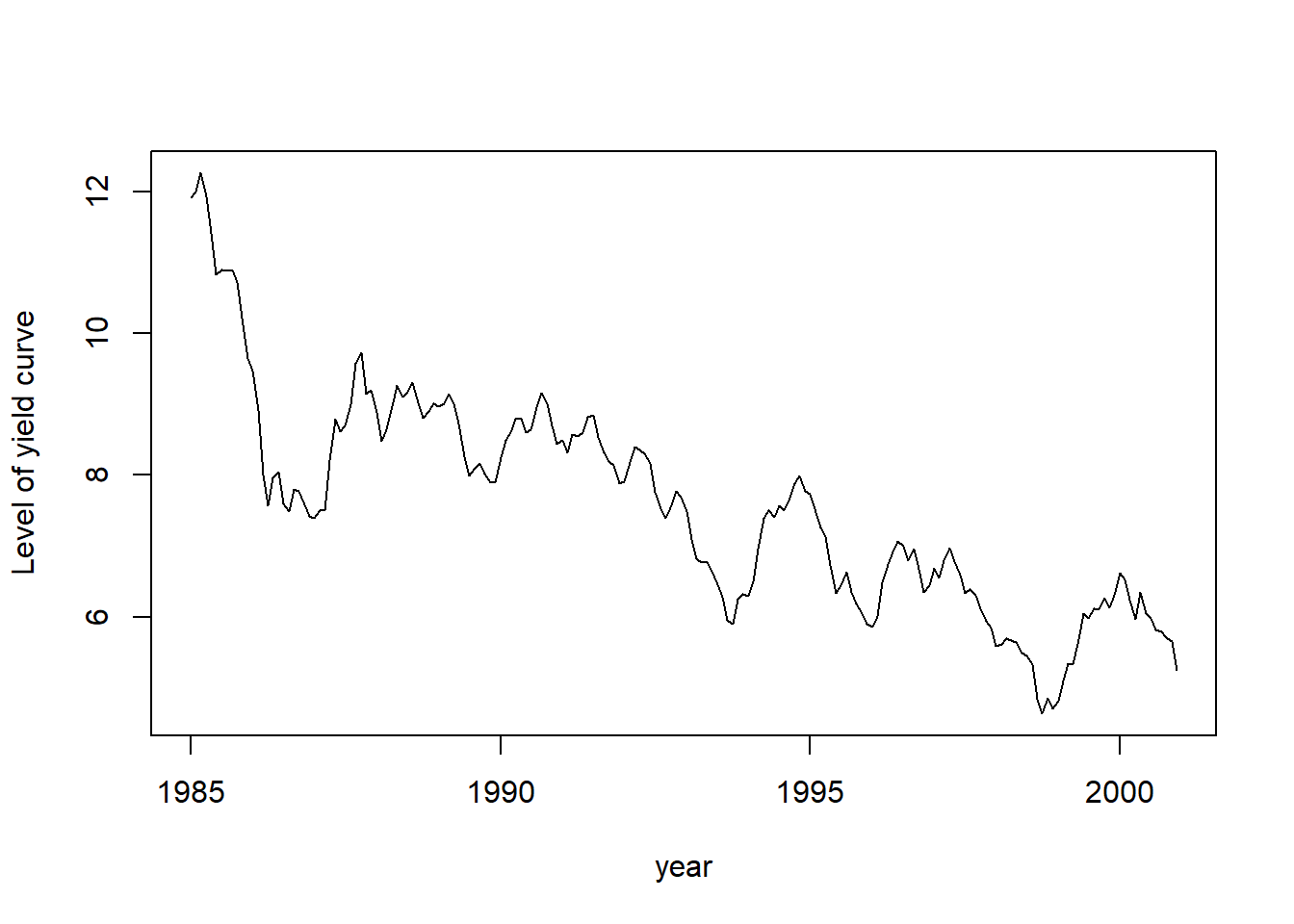
##  NULL

xts.yc <- FedYieldCurve["1984-12-31/2000-12-01"]
date.yc <- index(xts.yc)
y.yc <- coredata(xts.yc)
plot(xts.yc, multi.panel=FALSE)

需要自己指定模型的各个矩阵和初值。

## 保存自定义设置用的列表
spec <- list()
## 自己规定H矩阵（观测误差的方差阵）
spec$H_spec <- TRUE
## 状态向量维数，3个beta, 3个常数beta均值
spec$state_num <- 6

## 待估参数个数20个，包括：
##   1个 - $\lambda$
##   1个 - $\sigma_e^2$
##   6个 - $\Sigma_{\boldsymbol\eta}\ 3 \times 3$对称阵
##   9个 - $\Phi_{3\times 3}$矩阵
##   3个 - $\boldsymbol\mu$
spec$param_num <- 20

## 状态方程中$R$矩阵不起作用，方差结构直接编写在矩阵$Q$中
spec$R <- diag(1, 6, 6) # $I_6$

## 初始状态$\boldsymbol\alpha_1$的方差，元素都取为0，因为平稳
spec$P_inf <- matrix(0, 6, 6)

## 指定状态向量中不输出到观测的分量，
## 当压缩观测向量为标量时可提高计算效率
spec$state_only <- 4:6

模型要估计的参数（超参数）为\(\lambda\), \(\sigma_e^2\), 对称的\((\Sigma_{\boldsymbol\eta})_{3\times 3}\), \(\Phi_{3\times 3}\), \(\boldsymbol\mu_{3\times 1}\)。

对于必须取正值的参数，将其迭代计算的参数取自然对数后除以2。

对于要求正定的\(\Sigma_{\boldsymbol\eta}\)，将其做Cholesky分解\(LDL^T\)，其中\(D\)是对角元素为正值的对角阵， \(L\)是对角元素都等于1的下三角阵，用\(D\)和\(L\)的6个元素来作为待估参数。 statespacer提供了Cholesky函数将这样编码的参数转换成正定矩阵。

对向量自回归系数矩阵\(\Phi\)，要求其满足平稳性条件， statespacer包的CoeffARMA()函数用来改造输入的系数矩阵使其满足条件。

因为模型的各个重要矩阵、初始值等都需要编程计算而不是常数值，所以将自定义设定的sys_mat_fun元素设置为一个自定义函数：

spec$sys_mat_fun <- function(param) {
  ## 输入20个参数，具体意义见前面注释和说明
  
  # 8个期限，即$\tau$值
  maturity <- c(3, 6, 12, 24, 36, 60, 84, 120)
  
  # 从取了对数的参数值恢复$\lamabda$的值
  lambda <- exp(2 * param[1])
  
  # \sigma_e^2的值
  sigma2 <- exp(2 * param[2])
  
  # H是观测方程的误差向量的协方差阵参数。
  # 注意每个$t$对应的观测值是$8\times 1$向量。
  H <- sigma2 * diag(1, 8, 8)
  
  # 观测方程的Z矩阵，一个$8 \times 6$矩阵，
  # 前三列对应于$\beta_{1t}$, $\beta_{2t}$, $\beta_{3t}$
  # 后三列对应于$\beta$的三个均值，系数为0
  lambda_maturity <- lambda * maturity
  ze <- exp(-lambda_maturity)
  Z <- matrix(1, 8, 3)
  Z[, 2] <- (1 - ze) / lambda_maturity
  Z[, 3] <- Z[, 2] - ze
  
  # 状态方程的误差方差阵（$6 \times 6$）的左上角$3 \times 3$部分
  # 使用6个参数
  Q <- Cholesky(
    param = param[3:8], 
    decompositions = FALSE, 
    format = matrix(1, 3, 3))
  
  # 从输入的9个矩阵元素生成满足平稳性条件的向量自回归系数矩阵$\Phi$
  Tmat <- CoeffARMA(
    A = array(param[9:17], dim = c(3, 3, 1)),
    variance = Q,
    ar = 1, ma = 0)$ar[,,1]

  # 生成初始状态$\boldsymbol\alpha_1$的方差阵，确保其满足平稳性条件
  T_kronecker <- kronecker(Tmat, Tmat)
  Tinv <- solve(
    diag(1, dim(T_kronecker)[1], 
         dim(T_kronecker)[2]) - T_kronecker)
  vecQ <- matrix(Q)
  vecPstar <- Tinv %*% vecQ
  P_star <- matrix(vecPstar, dim(Tmat)[1], dim(Tmat)[2])


  ## 添加对应于常数均值的部分
  # 在观测方程的矩阵Z中增加对应于常数均值的3列
  Z <- cbind(Z, matrix(0, 8, 3)) 
  # 在状态方程的误差方差阵中增加对应于常数均值的部分，都是0
  Q <- BlockMatrix(Q, matrix(0, 3, 3)) 
  # 在6维的状态方程中，设置转移矩阵$T$
  Tmat <- cbind(Tmat, diag(1, 3, 3) - Tmat)
  Tmat <- rbind(Tmat, cbind(matrix(0, 3, 3), diag(1, 3, 3)))
  # 初始状态的方差阵中对应于常数均值部分方差和协方差为0
  P_star <- BlockMatrix(P_star, matrix(0, 3, 3))
  
  # $\beta$的均值是最后的3个待估参数，
  # 也作为$t=1$时$\beta$的初始分布均值
  a1 <- matrix(param[18:20], 6, 1) 
  
  # 函数返回模型所需的所有系统矩阵
  return(list(
    H = H,   # 观测误差随机向量的方差阵
    Z = Z,   # 观测方程的观测矩阵
    Tmat = Tmat, # 状态方程的状态转移矩阵
    Q = Q,   # 状态方程的误差随机向量的方差阵
    a1 = a1, # 初始状态的均值
    P_star = P_star)) # 初始状态的方差阵
}

为了从估计的参数（超参数）提取某些成分，可以提供一个transform_fun函数：

spec$transform_fun <- function(param) {
  lambda <- exp(2 * param[1])
  sigma2 <- exp(2 * param[2])
  means <- param[18:20]
  return(c(lambda, sigma2, means))
}

下面给20个参数设置算法迭代初值：

initial <- c(
  -1, # $0.5 \ln\lambda$
  -2, # $0.5 \ln\sigma_e^2$
  # $\Sigma_{\boldsymbol\eta}$的LDL分解中D的对角元素的0.5倍对数值
  -1, -1, -1, 
  # $\Sigma_{\boldsymbol\eta}$的LDL分解中L的元素值
  0, 0, 0, 
  # VAR(1)模型系数矩阵
  1, 0, 0, 
  0, 1, 0, 
  0, 0, 1, 
  # 三个beta的均值
  0, 0, 0)

进行模型拟合， statespacer()函数需要调用optim函数进行最大似然估计计算，可能需要消耗一定的时间：

fit <- statespacer(
  y = y.yc,
  self_spec_list = spec,
  collapse = TRUE,
  initial = initial,
  method = "BFGS",
  control = list(maxit = 200),
  verbose = TRUE)

## Starting the optimisation procedure at: 2023-05-26 09:32:19

## initial  value 18.089728 
## iter  10 value -6.160531
## iter  20 value -6.760946
## iter  30 value -6.953583
## iter  40 value -6.990606
## iter  50 value -6.996315
## iter  60 value -6.999004
## iter  70 value -7.002370
## iter  80 value -7.004278
## iter  90 value -7.005021
## iter 100 value -7.005174
## iter 110 value -7.005240
## iter 120 value -7.005375
## iter 130 value -7.005400
## iter 140 value -7.005430
## iter 150 value -7.005440
## iter 160 value -7.005462
## final  value -7.005470 
## converged

## Finished the optimisation procedure at: 2023-05-26 09:32:32

## Time difference of 13.2968471050262 secs

算法有可能在中间因矩阵不可逆而中断，这时可以修改初值。模型估计一次需要大约半分钟。将计算系统矩阵的函数改写为C++版本可能会加快速度。

平滑得到的\(\beta_{1t}\)的时间序列图形：

plot(date.yc, fit$smoothed$a[, 1], type = 'l', 
  xlab = "year", ylab = "Level of yield curve")

平滑得到的\(\beta_{2t}\)的时间序列图形：

plot(date.yc, fit$smoothed$a[, 2], type = 'l', 
  xlab = "year", ylab = "Slope of yield curve")

平滑得到的\(\beta_{3t}\)的时间序列图形：

plot(date.yc, fit$smoothed$a[, 3], type = 'l', 
  xlab = "year", ylab = "Shape of yield curve")

获取估计的参数：

parameters <- data.frame(
  Parameter = c("lambda", "sigma2", "mu1", "mu2", "mu3"), 
  Value = fit$system_matrices$self_spec,
  SE = fit$standard_errors$self_spec
)
knitr::kable(parameters, digits=4)

Parameter	Value	SE
lambda	0.0789	0.0017
sigma2	0.0035	0.0002
mu1	8.2277	2.0759
mu2	-2.2748	1.4364
mu3	-0.4256	0.7191

向量自回归系数矩阵：

fit$system_matrices$T$self_spec[1:3, 1:3]

##             [,1]        [,2]        [,3]
## [1,]  0.98488006 -0.01776100 0.005741521
## [2,] -0.01980538  0.94678326 0.062497259
## [3,] -0.03354339 -0.04024349 0.964429517

状态方程误差方差阵：

fit$system_matrices$Q$self_spec[1:3, 1:3]

##             [,1]        [,2]        [,3]
## [1,]  0.06723244 -0.05232934  0.06856474
## [2,] -0.05232934  0.07118337 -0.04047250
## [3,]  0.06856474 -0.04047250  0.24097759

28.5.8 四地点海豹数目调查建模

本例子来自(Holmes, Scheuerell, and Ward 2021)第7章。

28.5.8.1 问题介绍

MARSS包的例子数据集中，有一个数据集是美国西海岸5个采样点历年调查的海豹数目（对数值）。调查年份是1978-1999，不同采样点的数据缺失情况不同。

library(MARSS)
library(tidyverse)
pdat <- as.data.frame(MARSS::harborSealWA) |>
  pivot_longer(
    all_of(c("SJF", "SJI", "EBays", "PSnd", "HC")),
    names_to = "region",
    values_to = "value"  )
ggplot(pdat, aes(
  x = Year, y = value, col = region)) +
  geom_point() +
  geom_line() +
  labs(title = "Puget Sound Harbor Seal Surveys")

## Warning: Removed 39 rows containing missing values (geom_point).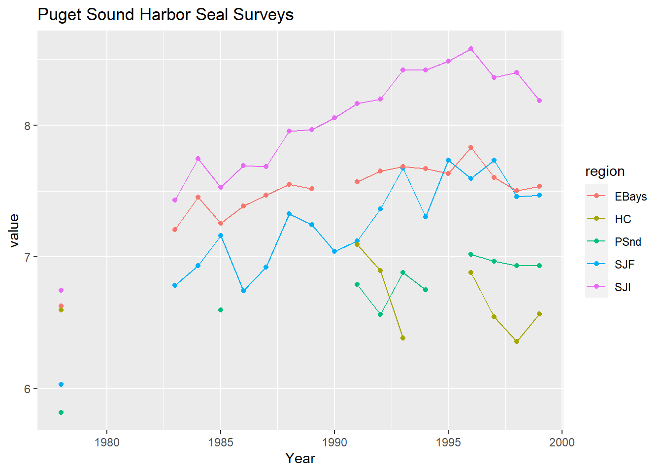

其中HC采样点比较独立，而且受到的外界影响与其它采样点区别较大，所以建模时去掉这个采样点。

下面对数据进行整理，最后保留4个采样点的逐年次序并转换为每个采样点占数据集一行的格式，这是MARSS需要的格式。

dat <- as.data.frame(MARSS::harborSealWA)
years <- dat[["Year"]]
d.seal <- dat |>
  select(-Year, -HC) |>
  t() 
colnames(d.seal) <- paste0(years)

28.5.8.2 单一总体的模型

假设所有的采样点的海豹来自同一个总体，其中的个体可以自由移动。设总体数据以几何速率增长。这时，设总体个数的对数值为\(x_t\)，则 \[ x_t = x_{t-1} + u + w_t, \ w_t \sim \text{N}(0,q) . \] 其中\(u\)是年对数增长率。

设四个采样点调查到的海豹数分别占总体数目的一个比例，我们不期望能估计这个比例本身，但是四个采样点观测到的海豹数的相对比例是可估的。所以设\(y_1, y_2, y_3, y_4\)是四个采样点观测到的海豹数目，则观测方程为 \[\begin{equation} \left[ \begin{array}{c} y_{1} \\ y_{2} \\ y_{3} \\ y_{4} \end{array} \right]_t = \left[ \begin{array}{c} 1\\ 1\\ 1\\ 1\end{array} \right] x_t + \left[ \begin{array}{c} 0 \\ a_2 \\ a_3 \\ a_4 \end{array} \right] + \left[ \begin{array}{c} v_{1} \\ v_{2} \\ v_{3} \\ v_{4} \end{array} \right]_t \tag{28.7} \end{equation}\] 注意数据是对数尺度的，以\(y_1\)为标准，总体数目\(x_t\)也是以\(y_1\)为一个相对标准的，并不会估计出总体的实际数目；然后，对数尺度上， \(y_2\)相对于\(y_1\)增加了\(a_2\)， \(y_3\)相对于\(y_1\)增加了\(a_3\)， \(y_4\)相对于\(y_1\)增加了\(a_4\)。设观测误差阵\(R\)是对角阵，对角元素不相等。

使用MARSS包的规定，模型指定如下：

seal.mod.0 <- list(
  B = matrix(1),   # 状态转移矩阵
  U = matrix("u"), # 状态漂移向量
  Q = matrix("q"), # 状态方程误差方差阵
  Z = matrix(1, 4, 1), # 观测方程矩阵
  A = "scaling",   # 观测方程各分量间的相对差值
  R = "diagonal and unequal", # 观测误差方差阵
  x0 = matrix("mu"), # 初值，未知常数
  tinitx = 0) # 模型从t=0开始

拟合模型：

seal.fit.0 <- MARSS(d.seal, model = seal.mod.0)

## Success! abstol and log-log tests passed at 32 iterations.
## Alert: conv.test.slope.tol is 0.5.
## Test with smaller values (<0.1) to ensure convergence.
## 
## MARSS fit is
## Estimation method: kem 
## Convergence test: conv.test.slope.tol = 0.5, abstol = 0.001
## Estimation converged in 32 iterations. 
## Log-likelihood: 21.62931 
## AIC: -23.25863   AICc: -19.02786   
##  
##                 Estimate
## A.SJI            0.79583
## A.EBays          0.27528
## A.PSnd          -0.54335
## R.(SJF,SJF)      0.02883
## R.(SJI,SJI)      0.03063
## R.(EBays,EBays)  0.01661
## R.(PSnd,PSnd)    0.01168
## U.u              0.05537
## Q.q              0.00642
## x0.mu            6.22810
## Initial states (x0) defined at t=0
## 
## Standard errors have not been calculated. 
## Use MARSSparamCIs to compute CIs and bias estimates.

可以通过拟合残差进行模型诊断。这里的残差是指向前一步预测结果的残差，即\(y_t - \hat y_t\)， \(\hat y_t\)是利用\(1:(t-1)\)的数据计算的预测值。

seal.resi <- function(seal.fit){
  opar <- par(mfrow = c(2, 2))
  on.exit(par(opar))
  resids <- MARSSresiduals(seal.fit, type = "tt1")
  for (i in 1:4) {
    plot(
      resids$model.residuals[i, ], 
      ylab = "model residuals", 
      xlab = "")
    abline(h = 0)
    title(rownames(d.seal)[i])
  }
}
seal.resi(seal.fit.0)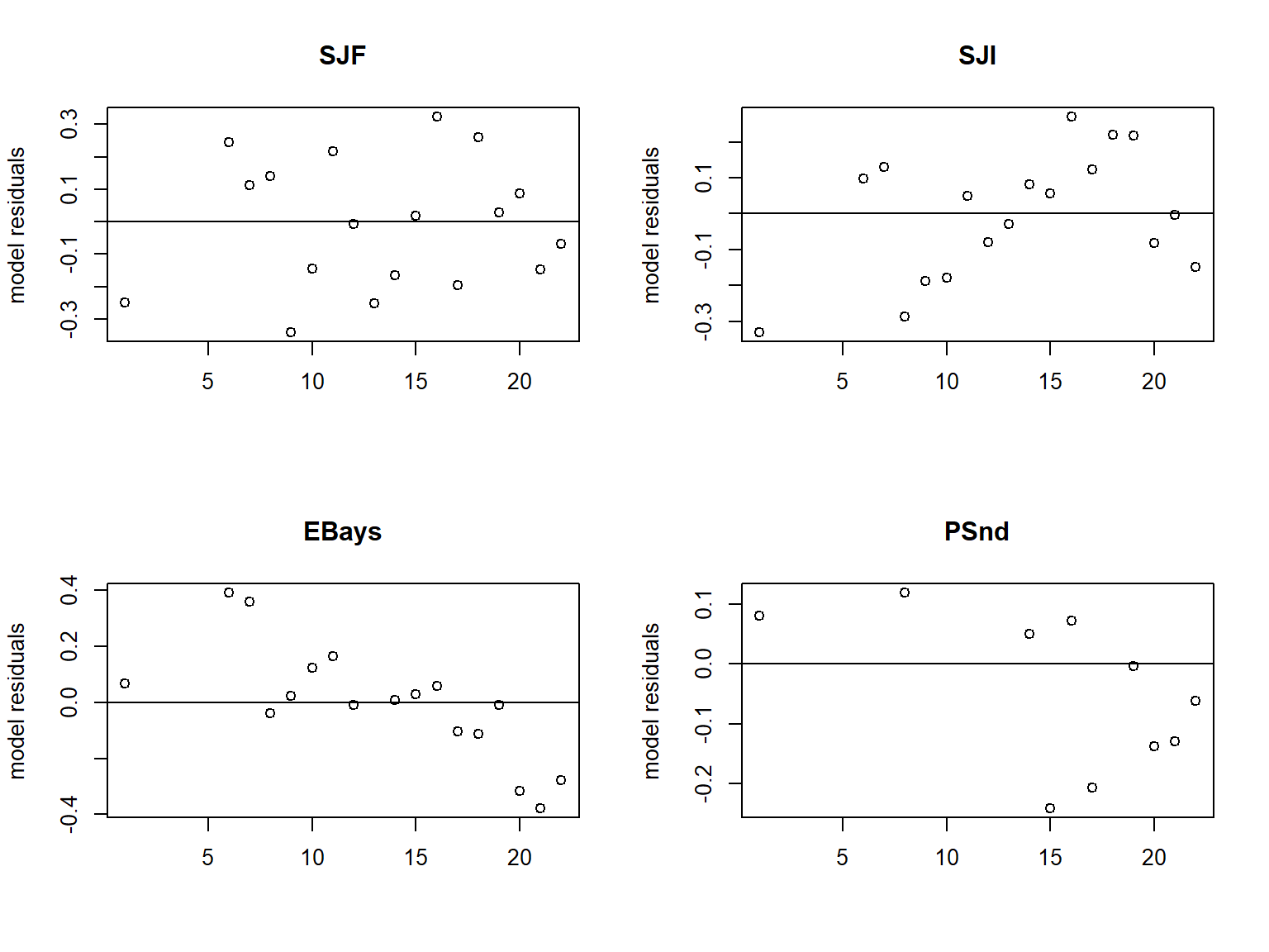

残差应该是没有规律的，但是这个模型的四个调查点的残差的都有一定规律。这说明四个调查点都来自同一个总体的假设不合理。

28.5.8.3 四个独立总体的模型

假设四个采样点的观测分别来自四个总体，且四个总体之间独立，但增长率相同，系统方程方差相等，即： \[\begin{equation} \begin{gathered} \begin{bmatrix}x_1\\x_2\\x_3\\x_4\end{bmatrix}_t = \begin{bmatrix} 1 & 0 & 0 & 0 \\ 0 & 1 & 0 & 0 \\ 0 & 0 & 1 & 0 \\ 0 & 0 & 0 & 1 \end{bmatrix} \begin{bmatrix}x_1\\x_2\\x_3\\x_4\end{bmatrix}_{t-1} + \begin{bmatrix}u\\u\\u\\u\end{bmatrix} + \begin{bmatrix}w_1\\w_2\\w_3\\w_4\end{bmatrix}_t \\ \textrm{ 其中 } \mathbf{w}_t \sim \,\text{MVN}\begin{pmatrix}0, \begin{bmatrix} q & 0 & 0 & 0 \\ 0 & q & 0 & 0\\ 0 & 0 & q & 0 \\ 0 & 0 & 0 & q \end{bmatrix}\end{pmatrix}\\ \begin{bmatrix}x_1\\x_2\\x_3\\x_4\end{bmatrix}_0 = \begin{bmatrix}\mu_1\\\mu_2\\\mu_3\\\mu_4\end{bmatrix}_t \end{gathered} \tag{28.8} \end{equation}\]

这时观测方程不再需要一个位移项\(a\)，变成 \[\begin{equation} \left[ \begin{array}{c} y_{1} \\ y_{2} \\ y_{3} \\ y_{4} \end{array} \right]_t = \begin{bmatrix} 1 & 0 & 0 & 0 \\ 0 & 1 & 0 & 0\\ 0 & 0 & 1 & 0 \\ 0 & 0 & 0 & 1 \end{bmatrix} \begin{bmatrix}x_1\\x_2\\x_3\\x_4\end{bmatrix}_t + \left[ \begin{array}{c} 0 \\ 0 \\ 0 \\ 0 \end{array} \right] + \left[ \begin{array}{c} v_{1} \\ v_{2} \\ v_{3} \\ v_{4} \end{array} \right]_t \tag{28.9} \end{equation}\] 仍设观测误差方差阵是对角阵，方差不相等。

设定MARSS模型：

seal.mod.1 <- list(
  B = "identity",  # 系统方程矩阵
  U = "equal",     # 系统方程位移项
  Q = "diagonal and equal", # 系统误差方差阵
  Z = "identity",  # 观测方程矩阵
  A = "zero",      # 观测方程位移项
  R = "diagonal and unequal", # 观测误差方差阵
  x0 = "unequal",  # 状态初值
  tinitx = 0)      # 系统从t=0计算

拟合模型：

seal.fit.1 <- MARSS(d.seal, model = seal.mod.1)

## Success! abstol and log-log tests passed at 24 iterations.
## Alert: conv.test.slope.tol is 0.5.
## Test with smaller values (<0.1) to ensure convergence.
## 
## MARSS fit is
## Estimation method: kem 
## Convergence test: conv.test.slope.tol = 0.5, abstol = 0.001
## Estimation converged in 24 iterations. 
## Log-likelihood: 23.21635 
## AIC: -26.43271   AICc: -22.20194   
##  
##                 Estimate
## R.(SJF,SJF)      0.02912
## R.(SJI,SJI)      0.00638
## R.(EBays,EBays)  0.00365
## R.(PSnd,PSnd)    0.00974
## U.1              0.05837
## Q.diag           0.00966
## x0.X.SJF         6.13673
## x0.X.SJI         6.73763
## x0.X.EBays       6.58977
## x0.X.PSnd        5.80029
## Initial states (x0) defined at t=0
## 
## Standard errors have not been calculated. 
## Use MARSSparamCIs to compute CIs and bias estimates.

28.5.8.4 四个相关总体的模型

在上面的模型中，假定四个总体的误差项是相关的，设\(Q\)矩阵形式为 \[ \mathbf{Q}=\begin{bmatrix} q & c & c & c \\ c & q & c & c\\ c & c & q & c \\ c & c & c & q \end{bmatrix} . \]

设定模型：

seal.mod.2 <- seal.mod.1
seal.mod.2$Q <- "equalvarcov"

估计：

seal.fit.2 <- MARSS(d.seal, model = seal.mod.2)

## Success! abstol and log-log tests passed at 31 iterations.
## Alert: conv.test.slope.tol is 0.5.
## Test with smaller values (<0.1) to ensure convergence.
## 
## MARSS fit is
## Estimation method: kem 
## Convergence test: conv.test.slope.tol = 0.5, abstol = 0.001
## Estimation converged in 31 iterations. 
## Log-likelihood: 34.09079 
## AIC: -46.18158   AICc: -41.00511   
##  
##                 Estimate
## R.(SJF,SJF)      0.02439
## R.(SJI,SJI)      0.00282
## R.(EBays,EBays)  0.00186
## R.(PSnd,PSnd)    0.00797
## U.1              0.05736
## Q.diag           0.01306
## Q.offdiag        0.01049
## x0.X.SJF         6.05525
## x0.X.SJI         6.70630
## x0.X.EBays       6.56580
## x0.X.PSnd        5.75608
## Initial states (x0) defined at t=0
## 
## Standard errors have not been calculated. 
## Use MARSSparamCIs to compute CIs and bias estimates.

比较三个模型的AICc：

c(seal.fit.0$AICc, seal.fit.1$AICc, seal.fit.2$AICc)

## [1] -19.02786 -22.20194 -41.00511

可见四个总体且总体之间相关的模型最优。

对最新的这个模型进行残差诊断：

seal.resi(seal.fit.2)

## MARSSresiduals.tt1 reported warnings. See msg element of returned residuals object.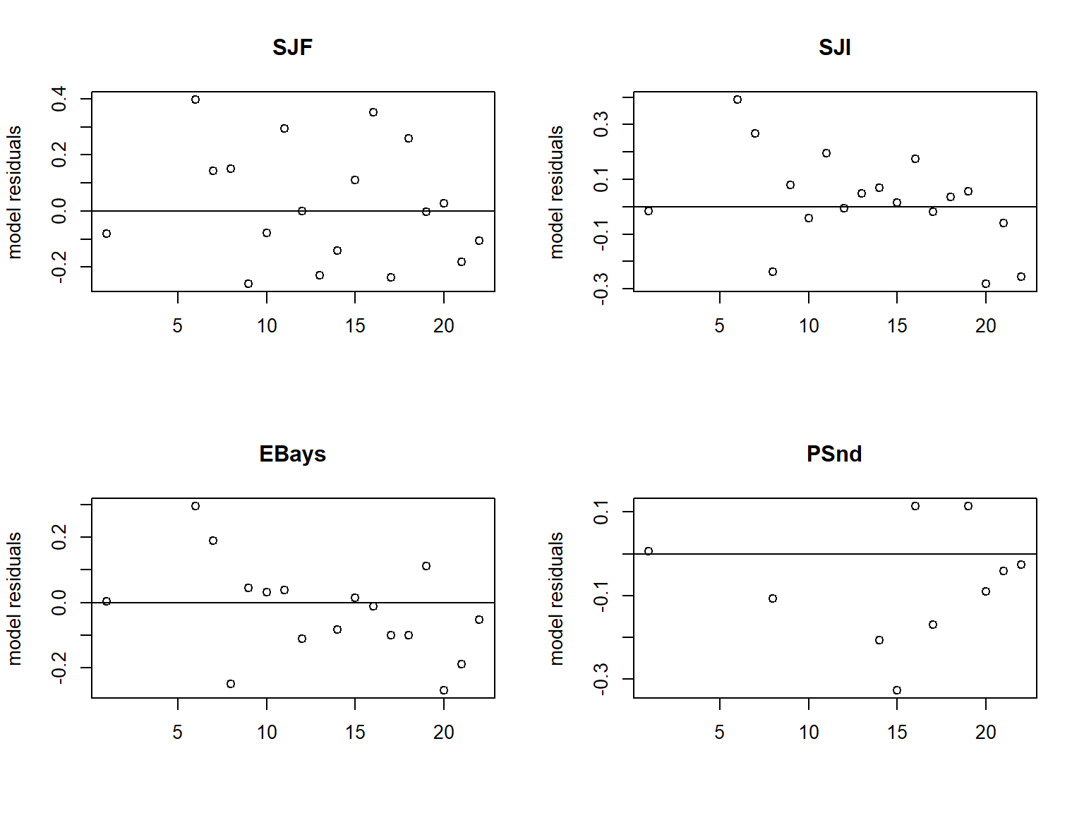

下面显示四个总体的对数数量（差一个常数位移值）估计值，是平滑结果：

seal.sta <- function(seal.fit){
  opar <- par(mfrow = c(2, 2))
  on.exit(par(opar))
  for (i in 1:4) {
    plot(years,
      seal.fit$states[i, ], 
      ylab = "log subpopulation estimate", 
      xlab = "", type="l")
    lines(
      years, 
      seal.fit$states[i, ] 
      - 1.96 * seal.fit$states.se[i, ], 
      type = "l", 
      lwd = 1, lty = 2, col = "red")    
    lines(
      years, 
      seal.fit$states[i, ] 
      + 1.96 * seal.fit$states.se[i, ], 
      type = "l", 
      lwd = 1, lty = 2, col = "red")    
    title(rownames(d.seal)[i])
  }
}
seal.sta(seal.fit.2)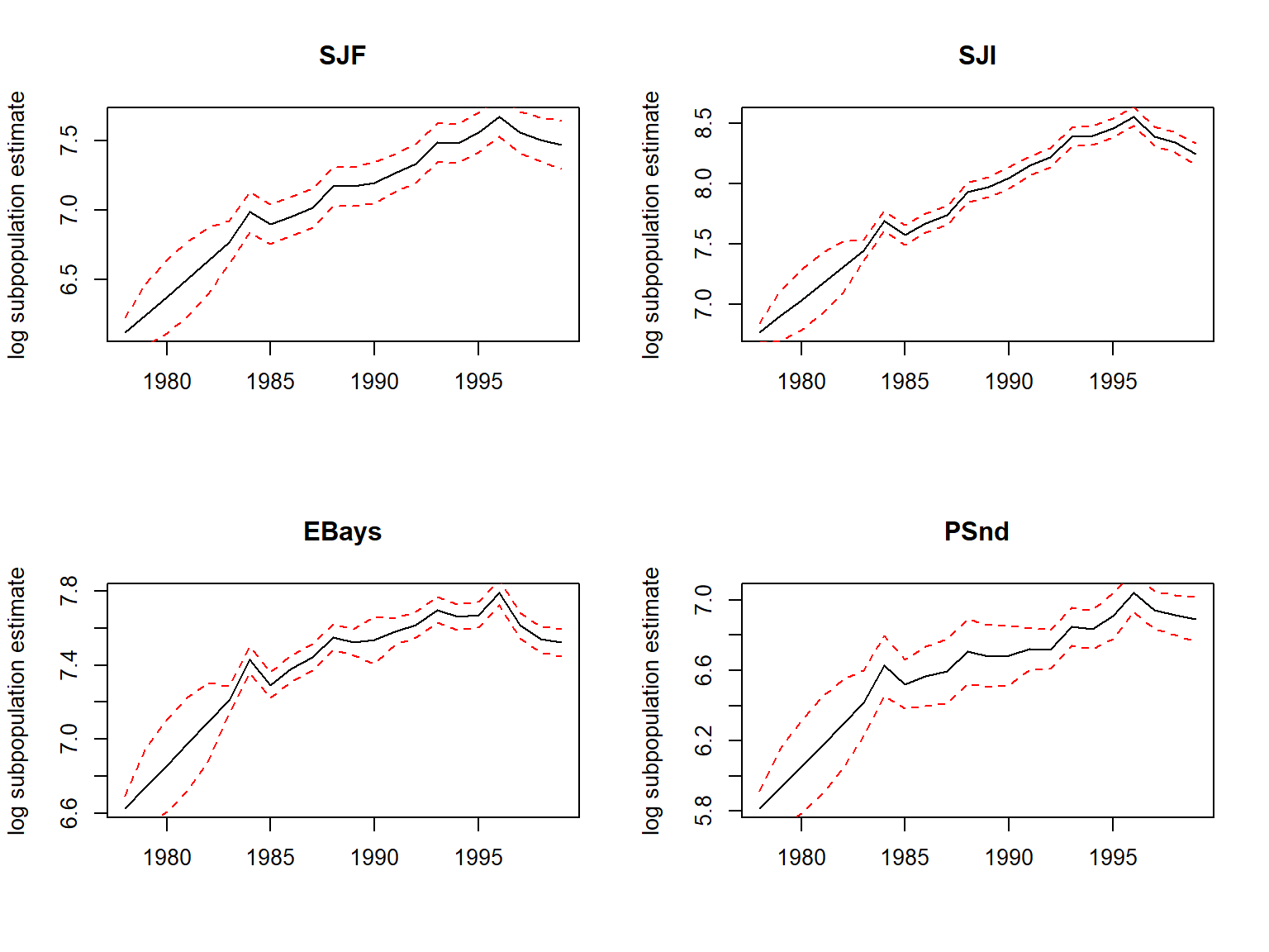

28.5.9 十一地点海豹数目调查建模

本例子来自(Holmes, Scheuerell, and Ward 2021)第7章。

28.5.9.1 问题介绍

MARSS包的harborSeal数据集包含了在美国西海岸的12个采样点逐年调查的海豹数据，采样年度为1975-2004，不同地点有不同的缺失年。

library(MARSS)
library(tidyverse)
pdat <- as.data.frame(MARSS::harborSeal) |>
  pivot_longer(
    -Year,
    names_to = "region",
    values_to = "value"  )
ggplot(pdat, aes(
  x = Year, y = value)) +
  geom_point() +
  facet_wrap(~region)

## Warning: Removed 163 rows containing missing values (geom_point).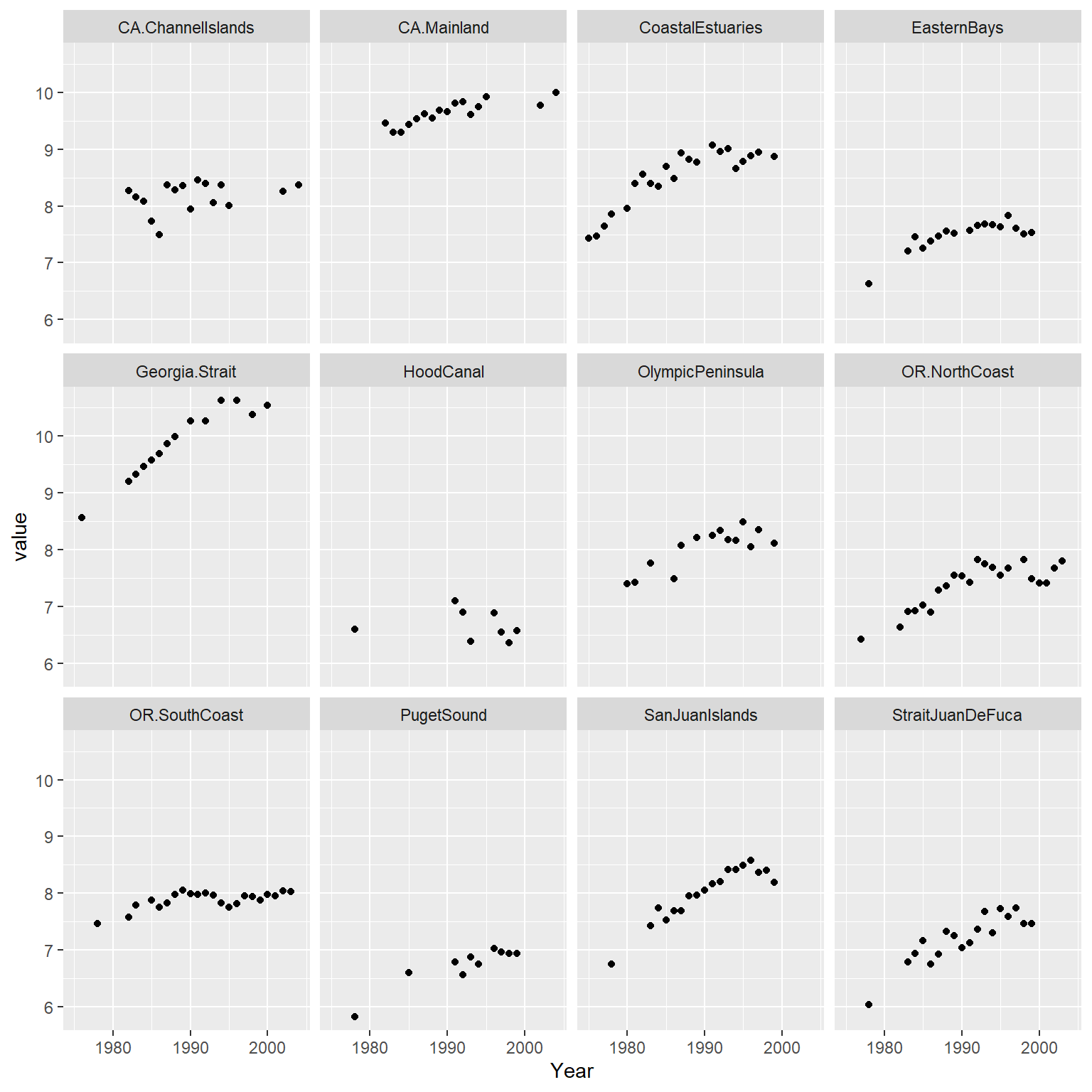

这12个采样点中HoolCanal的规律与其它采样点差别很大，建模中去掉。

dat <- MARSS::harborSeal
years <- dat[, "Year"]
good <- !(colnames(dat) %in% c("Year", "HoodCanal"))
sealData <- t(dat[, good])
colnames(sealData) <- years

28.5.9.2 状态方程的不同设置

对海豹总体个数，子总体组成，子总体的误差方差、相关性有不同的模型假设，应在这些模型之间进行比较选择。

H1: 三个子总体，按采样点的组织结构划分；
H2: 按内陆采样点和海岸采样点分成两个子总体；
H3: 按北部和南部分为两个子总体；
H4: 分为海岸北部，海岸南部，SJF和佐治亚海峡，Puget Sound地区共4个子总体；
H5: 仅一个总体；
H6: 每个调查点单独分属一个子总体。

这时，不同模型对应的观测方程矩阵\(Z\)的形式分别为：

\[ \begin{array}{rcccc} &H1&H2&H4&H5\\ &\text{pnw ps ca}&\text{coast pc}&\text{nc is ps sc}&\text{pan}\\ \hline \begin{array}{r}\text{Coastal Estuaries}\\ \text{Olympic Peninsula} \\ \text{Str. Juan de Fuca} \\ \text{San Juan Islands} \\ \text{Eastern Bays} \\ \text{Puget Sound} \\ \text{CA Mainland} \\ \text{CA Channel Islands} \\ \text{OR North Coast} \\ \text{OR South Coast} \\ \text{Georgia Strait} \end{array}& \begin{bmatrix} 1 & 0 & 0 \\ 1 & 0 & 0 \\ 0 & 1 & 0 \\ 0 & 1 & 0 \\ 0 & 1 & 0 \\ 0 & 1 & 0 \\ 0 & 0 & 1 \\ 0 & 0 & 1 \\ 1 & 0 & 0 \\ 1 & 0 & 0 \\ 0 & 1 & 0 \end{bmatrix}& \begin{bmatrix} 1 & 0 \\ 1 & 0 \\ 0 & 1 \\ 0 & 1 \\ 0 & 1 \\ 0 & 1 \\ 1 & 0 \\ 1 & 0 \\ 1 & 0 \\ 1 & 0 \\ 0 & 1 \end{bmatrix}& \begin{bmatrix} 1 & 0 & 0 & 0\\ 1 & 0 & 0 & 0\\ 0 & 1 & 0 & 0\\ 0 & 1 & 0 & 0\\ 0 & 0 & 1 & 0\\ 0 & 0 & 1 & 0\\ 0 & 0 & 0 & 1\\ 0 & 0 & 0 & 1\\ 1 & 0 & 0 & 0\\ 0 & 0 & 0 & 1\\ 0 & 1 & 0 & 0 \end{bmatrix}& \begin{bmatrix} 1 \\ 1 \\ 1 \\ 1 \\ 1 \\ 1 \\ 1 \\ 1 \\ 1 \\ 1 \\ 1 \end{bmatrix} \end{array} \]

H6的\(Z\)是一个单位阵。

可以先生成一个基本的MARSS设置列表，在此基础上修改。

hseal.mod <- list(
  B = "identity", # 这对应于各子总体为随机游动
  U = "unequal",  # 系统方程位移项
  Q = "equalvarcov", # 系统方程误差方差阵
  Z = "placeholder", # 观测方程矩阵，待定
  A = "scaling",     # 观测方程各子总体之间的相对差值
  R = "diagonal and equal", # 观测误差方差阵
  x0 = "unequal",    # 状态向量初值
  tinitx = 0         # 系统从t=0开始
)

下面将六种模型假设的每一个的\(Z\)矩阵都保存起来：

Z.models <- list(
  H1 = factor(c(
    "pnw", "pnw", rep("ps", 4), 
    "ca", "ca", "pnw", "pnw", "ps")),
  H2 = factor(c(
    rep("coast", 2), rep("ps", 4), 
    rep("coast", 4), "ps")),
  H3 = factor(c(
    rep("N", 6), "S", "S", 
    "N", "S", "N")),
  H4 = factor(c(
    "nc", "nc", "is", "is", 
    "ps", "ps", "sc", "sc", 
    "nc", "sc", "is")),
  H5 = factor(rep("pan", 11)),
  H6 = factor(1:11) )
names(Z.models) <-  c(
  "stock", "coast+PS", "N+S", 
  "NC+strait+PS+SC", "panmictic", "site")

28.5.9.3 拟合6个模型

这6个模型的系统方程误差方差阵都设置成了方差相等、协方差相等的形式。还应比较其它的设置。

下面的程序批量拟合6个模型，将结果保存到数据框中：

out.tab <- NULL
fits <- list()
for (i in seq_along(Z.models)) {
    hseal.mod$Z <- Z.models[[i]]
    fit <- MARSS::MARSS(
      sealData, model = hseal.mod, 
      silent = TRUE, 
      control = list(maxit = 1000))
    out <- data.frame(
      H = names(Z.models)[i], 
      logLik = fit$logLik, 
      AICc = fit$AICc, 
      num.param = fit$num.params, 
      m = length(unique(Z.models[[i]])), 
      num.iter = fit$numIter, 
      converged = !fit$convergence)
    out.tab <- rbind(out.tab, out)
    fits <- c(fits, list(fit))
}

拟合汇总表格：

knitr::kable(out.tab, digits=2)

H	logLik	AICc	num.param	m	num.iter	converged
stock	54.97	-72.37	17	3	347	TRUE
coast+PS	52.89	-70.62	16	2	294	TRUE
N+S	58.80	-82.43	16	2	70	TRUE
NC+strait+PS+SC	79.71	-119.40	18	4	433	TRUE
panmictic	39.07	-47.73	14	1	82	TRUE
site	84.86	-111.74	25	11	657	TRUE

如果按AICc指标比较，最好的是H4，分成4个子总体。

可以按AICc排序，并计算AICc差值（即减去最小值），然后用公式\(e^{-\frac{1}{2} \delta}\)计算“相对似然”，其中\(\delta\)是AICc差值，然后可以计算AICc权重，即将相对似然值归一化为总和等于1。

out.tab2 <- out.tab |>
  select(H, AICc) |>
  arrange(AICc) |>
  mutate(
    delta.AICc = AICc - min(AICc),
    rel.like = exp(-0.5*delta.AICc),
    AIC.weight = rel.like / sum(rel.like))
knitr::kable(out.tab2, digits = 3)

H	AICc	delta.AICc	rel.like	AIC.weight
NC+strait+PS+SC	-119.395	0.000	1.000	0.979
site	-111.743	7.652	0.022	0.021
N+S	-82.428	36.967	0.000	0.000
stock	-72.371	47.024	0.000	0.000
coast+PS	-70.618	48.777	0.000	0.000
panmictic	-47.730	71.665	0.000	0.000

28.5.10 就业人数回归模型

R的longley数据框包含了与就业有关的宏观经济数据。待完成。

28.5.11 蓝藻和蓝绿藻数据

此例来自MARSS手册。用来演示协变量回归。

数据是美国华盛顿湖浮游生物数据，取其中的绿藻(变量Greens)、蓝绿藻(变量Bluegreens)以及温度(变量Temp)、磷含量(变量TP)数据在1965-1974这10年的数据。绿藻、蓝绿藻含量数据中有缺失值。用温度、磷含量作为协变量（自变量）。

library(MARSS)
sc_fun <- \(da) scale(
  da, 
  center=apply(da, 2, \(x) mean(x, na.rm=TRUE)),
  scale=apply(da, 2, \(x) sd(x, na.rm=TRUE)))

# 蓝藻、蓝绿藻，二维的时间序列数据，
# 每列代表一个时间点，这是MARSS要求
dat <- lakeWAplanktonTrans |>
  as.data.frame() |>
  dplyr::filter(Year >= 1965 & Year < 1975) |>
  select(Greens, Bluegreens) |>
  sc_fun() |>
  t()

## 协变量，温度和磷含量
covariates <- lakeWAplanktonTrans |>
  as.data.frame() |>
  dplyr::filter(Year >= 1965 & Year < 1975) |>
  select(Temp, TP) |>
  scale() |>
  t()

da_algae <- cbind(t(dat), t(covariates)) |>
  as.data.frame()

plot(ts(da_algae, 
  start=c(1962,1), frequency=12))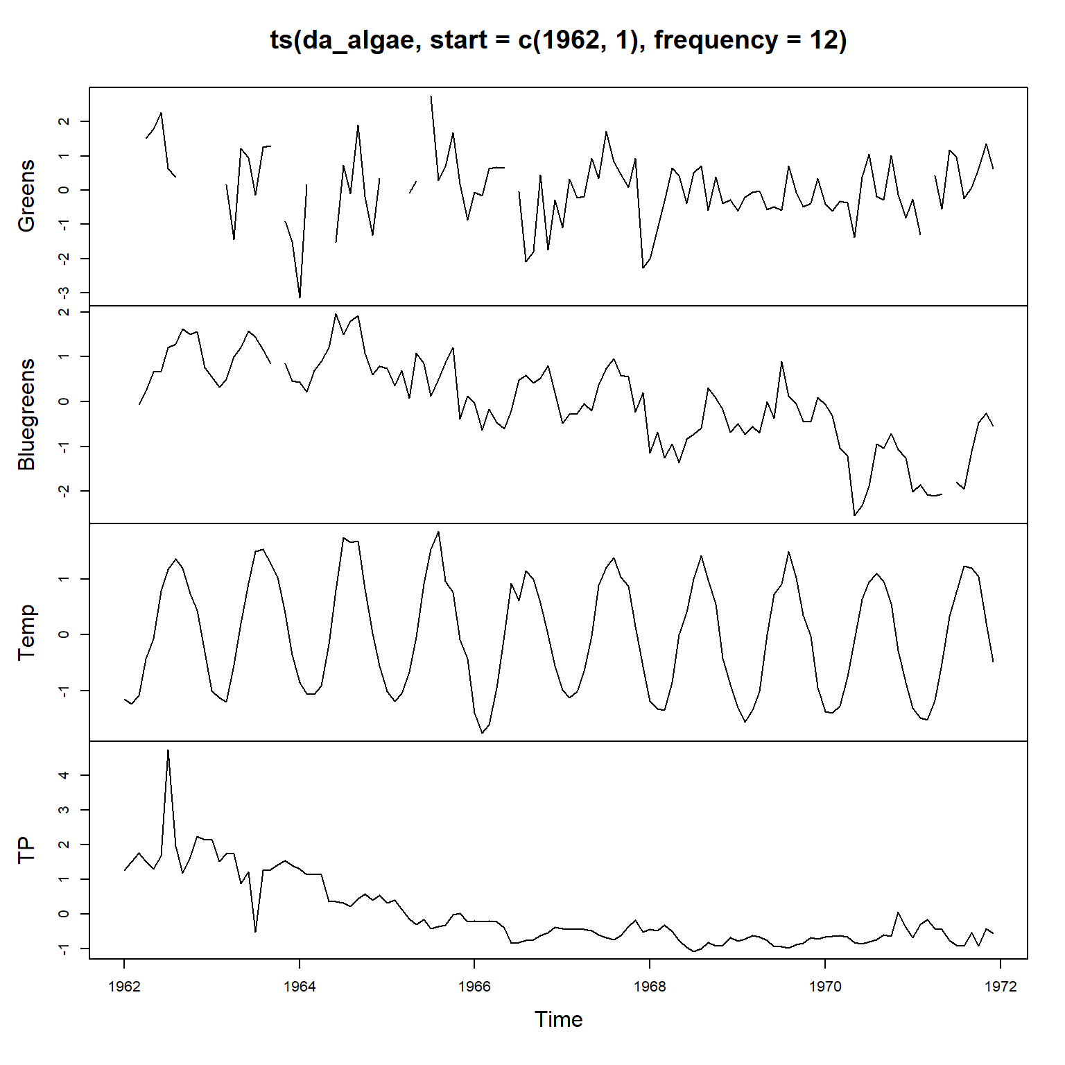

28.5.11.1 常系数多元线性回归模型

不考虑时间序列性质，仅以蓝藻、蓝绿藻含量为因变量，以温度、磷含量为自变量，作多元回归。这时系统方程的初值、误差方差阵都取为0矩阵，使得系统变量\(\boldsymbol x_t\)恒等于0。

alg_mod1 <- list(
  B = "identity",
  U = "zero",
  Q = "zero",
  Z = "identity",
  A = "zero",
  # 在观测方程中的协变量矩阵:
  d = covariates, 
  # 观测方程中的协变量回归系数矩阵:
  D = "unconstrained", 
  R = "diagonal and equal",
  x0 = "zero")
alg_fit1 <- MARSS(
  dat, model = alg_mod1)

## Success! algorithm run for 15 iterations. abstol and log-log tests passed.
## Alert: conv.test.slope.tol is 0.5.
## Test with smaller values (<0.1) to ensure convergence.
## 
## MARSS fit is
## Estimation method: kem 
## Convergence test: conv.test.slope.tol = 0.5, abstol = 0.001
## Algorithm ran 15 (=minit) iterations and convergence was reached. 
## Log-likelihood: -276.4287 
## AIC: 562.8573   AICc: 563.1351   
##  
##                     Estimate
## R.diag                 0.706
## D.(Greens,Temp)        0.367
## D.(Bluegreens,Temp)    0.392
## D.(Greens,TP)          0.058
## D.(Bluegreens,TP)      0.535
## Initial states (x0) defined at t=0
## 
## Standard errors have not been calculated. 
## Use MARSSparamCIs to compute CIs and bias estimates.

结果模型为(因为所有变量都标准化了，所以没有截距项) \[ \begin{pmatrix} \text{Greens}_t \\ \text{BlueGreens}_t \end{pmatrix} = \begin{pmatrix} 0.367 & 0.058 \\ 0.392 & 0.535 \end{pmatrix} \begin{pmatrix} \text{Temp}_t \\ \text{TP}_t \end{pmatrix} + \boldsymbol v_t, \] 其中\(\boldsymbol v_t\)的方差阵为对角阵且对角元素都等于\(0.706\)。

直接做多元回归的结果：

lm(Greens ~ -1 + Temp + TP, data=da_algae) |>
  summary()

## 
## Call:
## lm(formula = Greens ~ -1 + Temp + TP, data = da_algae)
## 
## Residuals:
##     Min      1Q  Median      3Q     Max 
## -2.8951 -0.5329  0.1322  0.5200  2.2228 
## 
## Coefficients:
##      Estimate Std. Error t value Pr(>|t|)    
## Temp  0.36740    0.09149   4.016 0.000113 ***
## TP    0.05801    0.09756   0.595 0.553378    
## ---
## Signif. codes:  0 '***' 0.001 '**' 0.01 '*' 0.05 '.' 0.1 ' ' 1
## 
## Residual standard error: 0.9325 on 103 degrees of freedom
##   (15 observations deleted due to missingness)
## Multiple R-squared:  0.1387, Adjusted R-squared:  0.122 
## F-statistic: 8.294 on 2 and 103 DF,  p-value: 0.0004572

lm(Bluegreens ~ -1 + Temp + TP, data=da_algae) |>
  summary()

## 
## Call:
## lm(formula = Bluegreens ~ -1 + Temp + TP, data = da_algae)
## 
## Residuals:
##      Min       1Q   Median       3Q      Max 
## -2.11028 -0.38226  0.06841  0.56525  1.46161 
## 
## Coefficients:
##      Estimate Std. Error t value Pr(>|t|)    
## Temp  0.39193    0.07096   5.523 2.10e-07 ***
## TP    0.53456    0.07162   7.464 1.74e-11 ***
## ---
## Signif. codes:  0 '***' 0.001 '**' 0.01 '*' 0.05 '.' 0.1 ' ' 1
## 
## Residual standard error: 0.7647 on 115 degrees of freedom
##   (3 observations deleted due to missingness)
## Multiple R-squared:  0.4202, Adjusted R-squared:  0.4101 
## F-statistic: 41.68 on 2 and 115 DF,  p-value: 2.44e-14

28.5.11.2 带有序列自相关误差项的回归

用系统方程表示回归模型中的误差项的相关性，使用两个一元零均值AR(1)模型，但无法检查参数估计结果是否平稳。

\[\begin{aligned} \boldsymbol x_t =& B \boldsymbol x_{t-1} + \boldsymbol w_t, \ \boldsymbol w_t \sim \text{N}(\boldsymbol 0, Q), \\ \boldsymbol y_t =& D_t \boldsymbol d_t + \boldsymbol x_t . \end{aligned}\]

其中\(\boldsymbol d_t\)是协变量，\(D_t\)是回归系数矩阵， \(B\)是对角阵，对角元素为AR(1)模型的自回归系数，观测方程没有观测误差。

alg_mod2 <- list(
  B = "diagonal and unequal",
  U = "zero",
  Q = "diagonal and unequal",
  Z = "identity",
  A = "zero",
  # 在观测方程中的协变量矩阵:
  d = covariates, 
  # 观测方程中的协变量回归系数矩阵:
  D = "unconstrained", 
  R = "diagonal and equal",
  x0 = "zero")
alg_fit2 <- MARSS(
  dat, model = alg_mod2)

## Success! abstol and log-log tests passed at 72 iterations.
## Alert: conv.test.slope.tol is 0.5.
## Test with smaller values (<0.1) to ensure convergence.
## 
## MARSS fit is
## Estimation method: kem 
## Convergence test: conv.test.slope.tol = 0.5, abstol = 0.001
## Estimation converged in 72 iterations. 
## Log-likelihood: -209.6348 
## AIC: 437.2695   AICc: 438.1186   
##  
##                               Estimate
## R.diag                          0.0449
## B.(X.Greens,X.Greens)           0.2442
## B.(X.Bluegreens,X.Bluegreens)   0.9183
## Q.(X.Greens,X.Greens)           0.7620
## Q.(X.Bluegreens,X.Bluegreens)   0.1234
## D.(Greens,Temp)                 0.3632
## D.(Bluegreens,Temp)             0.2542
## D.(Greens,TP)                   0.0349
## D.(Bluegreens,TP)               0.0608
## Initial states (x0) defined at t=0
## 
## Standard errors have not been calculated. 
## Use MARSSparamCIs to compute CIs and bias estimates.

模型为：

\[\begin{aligned} \text{Greens}_t =& 0.3632 \text{Temp}_t + 0.0349 \text{TP}_t + x_{1t}, \\ x_{1t} =& 0.2442 x_{1,t-1} + w_{1t}, \ w_{1t} \sim \text{N}(0, 0.7620); \\ \text{Bluegreens}_t =& 0.2542 \text{Temp}_t + 0.0608 \text{TP}_t + x_{2t}, \\ x_{2t} =& 0.9183 x_{2,t-1} + w_{2t}, \ w_{2t} \sim \text{N}(0, 0.1234) . \end{aligned}\]

实际操作上，还可以取\(B\)为单位阵，但这使得回归误差项为单位根过程，会破坏估计的稳定性。实际计算时效果也不好，得到的\(Q\)矩阵会很小，使得序列相关误差项变成可忽略的小值。

28.5.11.3 将主要模型表示在系统方程中

协变量的作用可以表示在观测方程中，也可以表示在系统方程中，令观测方程没有误差项。 \[ \boldsymbol x_t = \boldsymbol x_{t-1} + C \boldsymbol c_t + \boldsymbol w_t, \ \boldsymbol w_t \sim \text{N}(0, Q) . \] 而\(\boldsymbol y_t = \boldsymbol x_t\)。因变量的模型包括一个随机游动和协变量部分。

alg_mod3 <- list(
  B = "identity",
  U = "zero",
  # 在系统方程中的协变量矩阵:
  c = covariates, 
  # 系统方程中的协变量回归系数矩阵:
  C = "unconstrained", 
  Q = "equalvarcov",
  Z = "identity",
  A = "zero",
  R = "zero")
alg_fit3 <- MARSS(
  dat, model = alg_mod3)

## Success! algorithm run for 15 iterations. abstol and log-log tests passed.
## Alert: conv.test.slope.tol is 0.5.
## Test with smaller values (<0.1) to ensure convergence.
## 
## MARSS fit is
## Estimation method: kem 
## Convergence test: conv.test.slope.tol = 0.5, abstol = 0.001
## Algorithm ran 15 (=minit) iterations and convergence was reached. 
## Log-likelihood: -285.0732 
## AIC: 586.1465   AICc: 586.8225   
##  
##                       Estimate
## Q.diag                  0.7269
## Q.offdiag              -0.0210
## x0.X.Greens            -0.5189
## x0.X.Bluegreens        -0.2431
## C.(X.Greens,Temp)      -0.0434
## C.(X.Bluegreens,Temp)   0.0988
## C.(X.Greens,TP)        -0.0589
## C.(X.Bluegreens,TP)     0.0104
## Initial states (x0) defined at t=0
## 
## Standard errors have not been calculated. 
## Use MARSSparamCIs to compute CIs and bias estimates.

结果很不合理，且对数似然值变差了许多，这是因为藻类含量用随机游动是不合理的模型。

改用VAR(1)模型，但限制系数阵为对角阵：

alg_mod3b <- alg_mod3
alg_mod3b$B <- "diagonal and unequal"
alg_fit3b <- MARSS(
  dat, model = alg_mod3b)

## Success! algorithm run for 15 iterations. abstol and log-log tests passed.
## Alert: conv.test.slope.tol is 0.5.
## Test with smaller values (<0.1) to ensure convergence.
## 
## MARSS fit is
## Estimation method: kem 
## Convergence test: conv.test.slope.tol = 0.5, abstol = 0.001
## Algorithm ran 15 (=minit) iterations and convergence was reached. 
## Log-likelihood: -236.6106 
## AIC: 493.2211   AICc: 494.2638   
##  
##                               Estimate
## B.(X.Greens,X.Greens)           0.1981
## B.(X.Bluegreens,X.Bluegreens)   0.7672
## Q.diag                          0.4899
## Q.offdiag                      -0.0221
## x0.X.Greens                    -1.2915
## x0.X.Bluegreens                -0.4179
## C.(X.Greens,Temp)               0.2844
## C.(X.Bluegreens,Temp)           0.1655
## C.(X.Greens,TP)                 0.0332
## C.(X.Bluegreens,TP)             0.1340
## Initial states (x0) defined at t=0
## 
## Standard errors have not been calculated. 
## Use MARSSparamCIs to compute CIs and bias estimates.

这个模型结果比较合理，对数似然函数值也比较高，但是初值\(\boldsymbol x_0\)的估计为负值不合理；要求估计从\(t=1\)开始会出错，这是EM算法的固有设置，使用BFGS则会对\(Q\)矩阵有其它要求。

28.5.11.4 系统方程和观测方程都有误差项的模型

在前面的模型中对观测方程增加误差项。

\[\begin{aligned} \boldsymbol x_t =& B \boldsymbol x_{t-1} + C \boldsymbol c_t + \boldsymbol w_t, \ \boldsymbol w_t \sim \text{N}(0, Q) . \\ \boldsymbol y_t =& \boldsymbol x_t + \boldsymbol v_t, \ \boldsymbol v_t \sim \text{N}(0, R) . \end{aligned}\]

alg_mod4 <- list(
  B = "diagonal and unequal",
  U = "zero",
  # 在系统方程中的协变量矩阵:
  c = covariates, 
  # 系统方程中的协变量回归系数矩阵:
  C = "unconstrained", 
  Q = "diagonal and unequal",
  Z = "identity",
  A = "zero",
  R = "diagonal and unequal")
alg_fit4_em <- MARSS(
  dat, model = alg_mod4,
  control = list(maxit=20))

## Warning! Reached maxit before parameters converged. Maxit was 20.
##  neither abstol nor log-log convergence tests were passed.
## 
## MARSS fit is
## Estimation method: kem 
## Convergence test: conv.test.slope.tol = 0.5, abstol = 0.001
## WARNING: maxit reached at  20  iter before convergence.
##  Neither abstol nor log-log convergence test were passed.
##  The likelihood and params are not at the MLE values.
##  Try setting control$maxit higher.
## Log-likelihood: -208.4015 
## AIC: 440.803   AICc: 442.2958   
##  
##                               Estimate
## R.(Greens,Greens)               0.4674
## R.(Bluegreens,Bluegreens)       0.0413
## B.(X.Greens,X.Greens)           0.3176
## B.(X.Bluegreens,X.Bluegreens)   0.8254
## Q.(X.Greens,X.Greens)           0.3489
## Q.(X.Bluegreens,X.Bluegreens)   0.1246
## x0.X.Greens                    -0.8270
## x0.X.Bluegreens                -0.3351
## C.(X.Greens,Temp)               0.2262
## C.(X.Bluegreens,Temp)           0.1506
## C.(X.Greens,TP)                 0.0279
## C.(X.Bluegreens,TP)             0.1049
## Initial states (x0) defined at t=0
## 
## Standard errors have not been calculated. 
## Use MARSSparamCIs to compute CIs and bias estimates.
## 
## Convergence warnings
##  Warning: the  x0.X.Greens  parameter value has not converged.
##  Warning: the  logLik  parameter value has not converged.
##  Type MARSSinfo("convergence") for more info on this warning.

alg_fit4 <- MARSS(
  dat, model = alg_mod4,
  inits = alg_fit4_em$par, 
  method = "BFGS")

## Success! Converged in 30 iterations.
## Function MARSSkfas used for likelihood calculation.
## 
## MARSS fit is
## Estimation method: BFGS 
## Estimation converged in 30 iterations. 
## Log-likelihood: -207.2771 
## AIC: 438.5542   AICc: 440.047   
##  
##                                Estimate
## R.(Greens,Greens)              3.67e-05
## R.(Bluegreens,Bluegreens)      3.23e-02
## B.(X.Greens,X.Greens)          1.88e-01
## B.(X.Bluegreens,X.Bluegreens)  8.17e-01
## Q.(X.Greens,X.Greens)          8.25e-01
## Q.(X.Bluegreens,X.Bluegreens)  1.36e-01
## x0.X.Greens                   -1.40e+00
## x0.X.Bluegreens               -3.52e-01
## C.(X.Greens,Temp)              2.89e-01
## C.(X.Bluegreens,Temp)          1.53e-01
## C.(X.Greens,TP)                3.43e-02
## C.(X.Bluegreens,TP)            1.09e-01
## Initial states (x0) defined at t=0
## 
## Standard errors have not been calculated. 
## Use MARSSparamCIs to compute CIs and bias estimates.

观测误差方差较小，没有起太大作用。

28.5.12 Seatbelts数据建模

R的datasets包的Seatbelts数据是一个多元时间序列，为月度数据，保存了英国1969年到1984年与道路交通事故有关的数据。分量含义：

DriversKilled: 小汽车交通事故死亡人数。
drivers: 小汽车交通事故死亡以及重伤人数。
front: 前排驾乘人员死亡和重伤人数。
rear: 后排乘客死亡和重伤人数。
kms: 已行驶里程。
PetroPrice: 汽油价格。
VanKilled: 小型厢式载货汽车司机死亡人数。
law: 强制安全带法律是否已实施的0-1变量，从1983-01-31起实行。

28.5.12.1 数据预处理

因为取正值的变量建模时比较受限制，所以将这些变量取对数值。

library(statespacer)
library(datasets)
da <- as.xts(Seatbelts) |> coredata()
for(v in c("drivers", "front", "rear", "PetrolPrice", "kms"))
  da[, v] <- log(da[,v])

28.5.12.2 确定性水平和季节项、有回归自变量的一元模型

以小汽车交通事故死亡、重伤人数（对数值）为因变量。以汽油价格（对数值）和是否实行了安全带法令为自变量。模型为 \[\begin{aligned} y_t =& \mu_t + \gamma_t + \beta_1 x_{1t} + \beta_2 x_{2t} + e_t, \\ \mu_{t+1} =& \mu_{t}, \\ \gamma_{t+1} =& -\sum_{j=1}^{11} \gamma_{t+1-j} . \end{aligned}\]

y <- cbind(da[,"drivers"])
ssmr1 <- statespacer(
  y = y, # 因变量
  local_level_ind = TRUE, # 是否有局部水平项
  # 设置局部水平项误差方差为零，从而非随机:
  format_level = matrix(0), 
  BSM_vec = 12, # 季节项的周期
  # 设置季节项误差项方差为零，从而非随机:
  format_BSM_list = list(matrix(0)), 
  # 添加的外生自变量，每个因变量分量需要输入一个自变量矩阵，
  # 所以即使是一元因变量也需要用列表
  addvar_list = list(as.matrix(
    da[, c("PetrolPrice", "law")])),
  method = "BFGS",
  # 唯一的方差参数$\sigma_e^2$的初值，
  # 算法中使用其对数值的2倍以确保取正值
  initial = 0.5 * log(var(c(y))), 
  verbose = TRUE)

## Starting the optimisation procedure at: 2023-05-26 09:26:42

## initial  value -0.443442 
## final  value -0.735372 
## converged

## Finished the optimisation procedure at: 2023-05-26 09:26:42

## Time difference of 0.0513920783996582 secs

观测误差方差\(\sigma_e^2\)估计：

ssmr1$system_matrices$H$H[1,1]

## [1] 0.007402481

非随机的局部水平\(\mu\)的平滑估计：

ssmr1$smoothed$level[1,1]

## [1] 6.401571

第一个自变量，即汽油价格对数值，的回归系数：

ssmr1$smoothed$addvar_coeff[1, 1]

## [1] -0.4521301

第二个自变量，即强制安全带法令是否实行，的回归系数，和相应标准误差估计， t统计量值：

c(coef = ssmr1$smoothed$addvar_coeff[1, 2],
  se = ssmr1$smoothed$addvar_coeff_se[1, 2],
  tstat = ssmr1$smoothed$addvar_coeff[1, 2] /
    ssmr1$smoothed$addvar_coeff_se[1, 2])

##        coef          se       tstat 
## -0.19713947  0.02072792 -9.51081922

由此计算的法令影响的t统计量低于\(-2\)，在0.05水平下显著，认为法令生效后水平伤亡水平显著降低。

下面将原始数据与平滑拟合结果（包括局部水平、季节项与自变量作用）作图：

plot(Seatbelts[, c("drivers")], type = "l", ylim = c(6.95, 8.1),
     lwd=2,
     xlab = "year", ylab = "logarithm of drivers")
lines(seq(tsp(Seatbelts)[1], tsp(Seatbelts)[2], 1/tsp(Seatbelts)[3]), 
      ssmr1$smoothed$level
      + ssmr1$smoothed$BSM12
      + ssmr1$smoothed$addvar, 
      type = 'l', col = "red",
      lty=3)
legend("topright",
  c("log(drivers)", "Smoothed fit"), 
  lty = c(1,3), lwd=c(2, 1), col = c("black", "red"))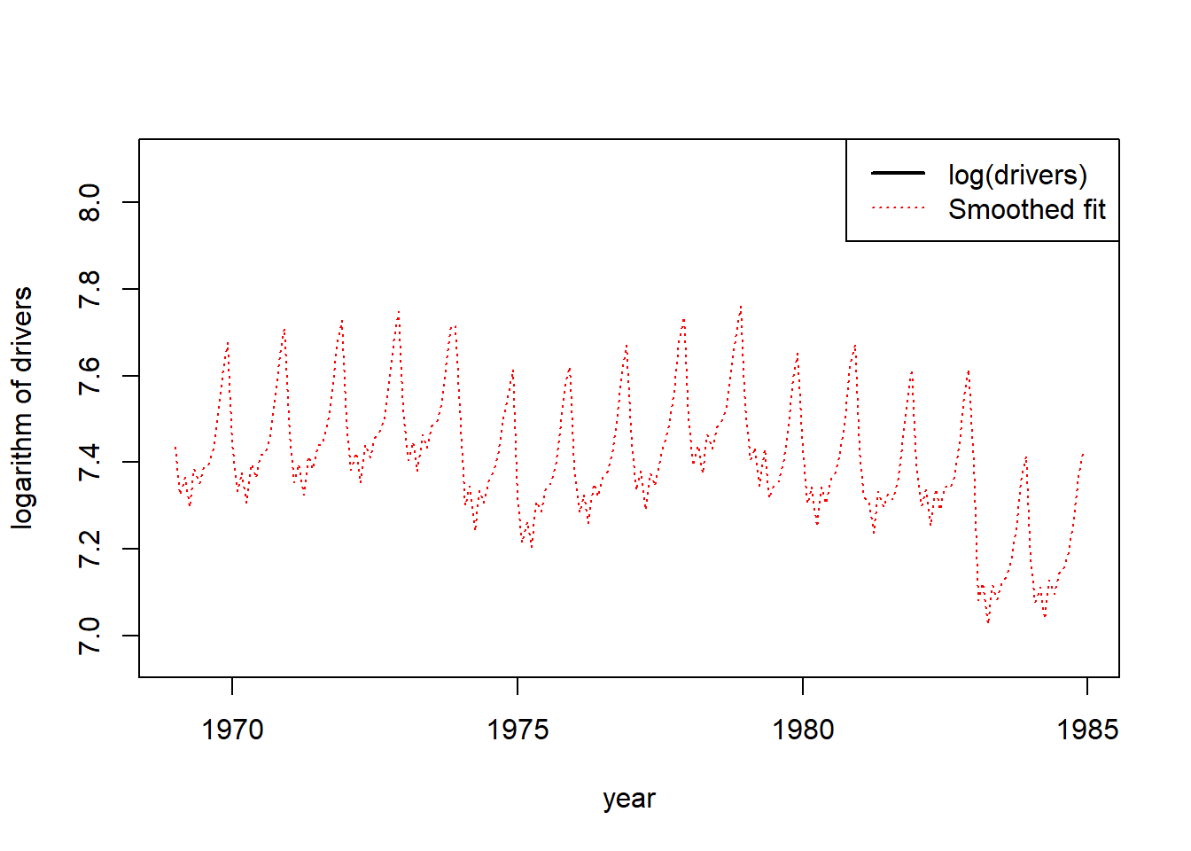

28.5.12.3 随机水平和季节项、有回归自变量的一元模型

模型为 \[\begin{aligned} y_t =& \mu_t + \gamma_t + \beta_1 x_{1t} + \beta_2 x_{2t} + e_t, \\ \mu_{t+1} =& \mu_{t} + \eta_t, \\ \gamma_{t+1} =& -\sum_{j=1}^{11} \gamma_{t+1-j} + \zeta_t . \end{aligned}\]

和确定性的\(\mu\), \(\gamma_t\)相比，程序只需将零方差改为非零方差：

y <- cbind(da[,"drivers"])
ssmr2 <- statespacer(
  y = y, # 因变量
  local_level_ind = TRUE, # 是否有局部水平项
  # 设置局部水平项误差方差为非零，从而随机:
  format_level = matrix(1), 
  BSM_vec = 12, # 季节项的周期
  # 设置季节项误差项方差为零，从而随机:
  format_BSM_list = list(matrix(1)), 
  # 添加的外生自变量，每个因变量分量需要输入一个自变量矩阵，
  # 所以即使是一元因变量也需要用列表
  addvar_list = list(as.matrix(da[, c("PetrolPrice", "law")])),
  method = "BFGS",
  # 唯一的方差参数$\sigma_e^2$的初值，
  # 算法中使用其对数值的2倍以确保取正值
  initial = log(var(as.vector(y))), 
  verbose = TRUE)

## Warning: Number of initial parameters is less than the required amount of
## parameters (3), recycling the initial parameters the required amount of times.

## Starting the optimisation procedure at: 2023-05-26 09:26:42

## initial  value -0.172423 
## iter  10 value -0.893962
## iter  20 value -0.915493
## iter  30 value -0.915515
## final  value -0.915517 
## converged

## Finished the optimisation procedure at: 2023-05-26 09:26:43

## Time difference of 0.770241975784302 secs

程序中还修改了原来的迭代初值，原来的迭代初值导致迭代过程出错。初值需要三个方差参数对应的初值，这里只给了一个初值，就重复利用。

估计结果：

## 观测误差方差估计
ssmr2$system_matrices$H$H[1,1]

## [1] 0.003786183

## 局部水平的系统方程的误差方差估计
ssmr2$system_matrices$Q$level[1,1]

## [1] 0.0002676875

## 季节项的系统方程的误差方差估计
ssmr2$system_matrices$Q$BSM12[1,1]

## [1] 1.161438e-06

## 关于汽油价格对数值这一自变量的回归系数估计
ssmr2$smoothed$addvar_coeff[1, 1]

## [1] -0.2913944

第二个自变量，即强制安全带法令是否实行，的回归系数，和相应标准误差估计， t统计量值：

c(coef = ssmr2$smoothed$addvar_coeff[1, 2],
  se = ssmr2$smoothed$addvar_coeff_se[1, 2],
  tstat = ssmr2$smoothed$addvar_coeff[1, 2] /
    ssmr2$smoothed$addvar_coeff_se[1, 2])

##        coef          se       tstat 
## -0.23773735  0.04631717 -5.13281209

结果表明法令生效后伤亡水平显著降低。

原始数据与拟合结果（拟合结果是平滑结果，利用了平滑的局部水平与自变量线性组合）：

plot(Seatbelts[, c("drivers")], type = "l", 
     ylim = c(6.95, 8.1),
     lwd=2,
     xlab = "year", ylab = "logarithm of drivers")
lines(seq(tsp(Seatbelts)[1], tsp(Seatbelts)[2], 1/tsp(Seatbelts)[3]), 
      ssmr2$smoothed$level 
      + ssmr2$smoothed$BSM12
      + ssmr2$smoothed$addvar, 
      lwd=1, lty=3,
      type = 'l', col = "red")
legend("topright",
  c("log(drivers)", "smoothed fit"), 
  lty = c(1,3), lwd=c(2, 1), col = c("black", "red"))

与非随机的水平和季节项的拟合结果比较，随机的水平和季节项使得拟合结果更贴近原始数据。

实际上，从季节项的系统方程的误差方差\(10^{-6}\)级别可以看出季节项的随机性很小，下面作平滑估计的季节项图形：

plot(seq(tsp(Seatbelts)[1], tsp(Seatbelts)[2], 1/tsp(Seatbelts)[3]), 
     ssmr2$smoothed$BSM12,
     type = "l", ylim = c(-0.2, 0.3),
     xlab = "year", ylab = "stochastic seasonal")
abline(h = 0)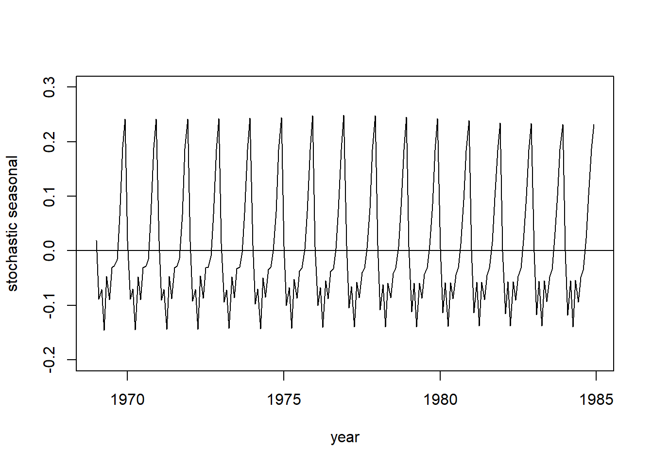

我们将随机的季节项改为非随机：

y <- cbind(da[,"drivers"])
ssmr3 <- statespacer(
  y = y, # 因变量
  local_level_ind = TRUE, # 是否有局部水平项
  # 设置局部水平项误差方差为非零，从而随机:
  format_level = matrix(1), 
  BSM_vec = 12, # 季节项的周期
  # 设置季节项误差项方差为零，从而非随机:
  format_BSM_list = list(matrix(0)), 
  # 添加的外生自变量，每个因变量分量需要输入一个自变量矩阵，
  # 所以即使是一元因变量也需要用列表
  addvar_list = list(as.matrix(
    da[, c("PetrolPrice", "law")])),
  method = "BFGS",
  # 唯一的方差参数$\sigma_e^2$的初值，
  # 算法中使用其对数值的2倍以确保取正值
  initial = log(var(c(y))), 
  verbose = TRUE)

## Warning: Number of initial parameters is less than the required amount of
## parameters (2), recycling the initial parameters the required amount of times.

## Starting the optimisation procedure at: 2023-05-26 09:26:44

## initial  value -0.577129 
## iter  10 value -0.912856
## final  value -0.912859 
## converged

## Finished the optimisation procedure at: 2023-05-26 09:26:44

## Time difference of 0.247884035110474 secs

估计结果：

## 观测误差方差估计
ssmr3$system_matrices$H$H[1,1]

## [1] 0.004033516

## 局部水平的系统方程的误差方差估计
ssmr3$system_matrices$Q$level[1,1]

## [1] 0.0002681651

## 关于汽油价格对数值这一自变量的回归系数估计
ssmr3$smoothed$addvar_coeff[1, 1]

## [1] -0.2767301

第二个自变量，即强制安全带法令是否实行，的回归系数，和相应标准误差估计， t统计量值：

c(coef = ssmr3$smoothed$addvar_coeff[1, 2],
  se = ssmr3$smoothed$addvar_coeff_se[1, 2],
  tstat = ssmr3$smoothed$addvar_coeff[1, 2] /
    ssmr3$smoothed$addvar_coeff_se[1, 2])

##       coef         se      tstat 
## -0.2375904  0.0464483 -5.1151578

结果表明法令生效后伤亡水平显著降低。

比较三个模型的AIC：

c(ssmr1$diagnostics$AIC, 
  ssmr2$diagnostics$AIC, 
  ssmr3$diagnostics$AIC)

## [1] -1.314494 -1.653950 -1.659052

第三个模型的AIC最小。

28.5.12.4 前后座驾乘人员同时建模的二元模型

考虑前座驾乘人员和后座乘客死亡、重伤人数对数的二元模型，都以汽油价格对数值、行驶里程对数值和安全带法令为自变量。

y <- da[,c("front", "rear")]
Xmat <- da[,c("PetrolPrice", "kms", "law")]
ssmr4 <- statespacer(y = y, # 输入数据是两列矩阵，二元时间序列
  # 观测方程误差项方差阵格式，这里是无限制的二阶方差阵
  H_format = matrix(1,2,2),
  local_level_ind = TRUE,
  # 局部水平的系统方程的误差项方差设置，无限制：
  format_level = matrix(1, 2, 2), 
  BSM_vec = 12,
  # 季节项的系统方程的误差项方差设置，设置为零，表示非随机季节项
  format_BSM_list = list(matrix(0, 2, 2)),
  # 每个因变量所需的自变量矩阵：
  addvar_list = list(Xmat, Xmat),
  method = "BFGS",
  initial = 0.5 * log(diag(var(y))),
  verbose = TRUE)

## Warning: Number of initial parameters is less than the required amount of
## parameters (6), recycling the initial parameters the required amount of times.

## Starting the optimisation procedure at: 2023-05-26 09:26:45

## initial  value 0.389588 
## iter  10 value -1.583525
## iter  20 value -1.676129
## iter  30 value -1.676530
## final  value -1.676537 
## converged

## Finished the optimisation procedure at: 2023-05-26 09:26:56

## Time difference of 11.4353930950165 secs

观测方程误差方差阵估计：

ssmr4$system_matrices$H$H

##             [,1]        [,2]
## [1,] 0.005402166 0.004449533
## [2,] 0.004449533 0.008566858

局部水平的系统方程的误差方差阵估计：

ssmr4$system_matrices$Q$level

##              [,1]         [,2]
## [1,] 0.0002556392 0.0002247045
## [2,] 0.0002247045 0.0002319561

6个回归系数及相应的t统计量：

data.frame(
  x1 = c("front PetrolPrice", "front kms", "front law", 
    "rear PetrolPrice", "rear kms", "rear law"),
  x2 = ssmr4$smoothed$addvar_coeff[1,],
  x3 = ssmr4$smoothed$addvar_coeff[1,] 
  / ssmr4$smoothed$addvar_coeff_se[1,]) |>
  knitr::kable(
    col.names=c("", "Coef", "t stat"),
    digits=4  )

	Coef	t stat
front PetrolPrice	-0.3076	-2.8986
front kms	0.1518	1.1678
front law	-0.3370	-6.8466
rear PetrolPrice	-0.0858	-0.7639
rear kms	0.5504	3.7927
rear law	0.0009	0.0171

与常识一致的是，后排乘客的伤亡数并不受安全带法令的影响。汽油价格上升对前排驾乘人员伤亡数有抑制作用。行驶里程数对前排驾乘人员伤亡数没有显著影响，但对后排乘客伤亡有正向的影响。

程序中还可以限制某个方差阵的秩，比如取format_level为 \[ \begin{pmatrix} 1 & 0 \\ 1 & 0 \end{pmatrix} \] 可以限制水平的系统方差的误差方差阵（\(2 \times 2\)方差阵）为秩等于1。

B 参考文献

Beijers, Dylan. 2020. statespacer: State Space Modelling in r. https://dylanb95.github.io/statespacer/.

Durbin, James, and Siem Jan Koopman. 2012. Time Series Analysis by State Space Methods. 2nd ed. Oxford University Press.

Holmes, E. E., M. D. Scheuerell, and E. J. Ward. 2021. Applied Time Series Analysis for Fisheries and Environmental Sciences. https://atsa-es.github.io/atsa-labs/.

Tsay, Ruey S. 2010. Analysis of Financial Time Series. 3rd Ed. John Wiley & Sons, Inc.

West, Mike, and Jeff Harrison. 1997. Bayesian Forecasting and Dynamic Models. Springer-Verlag. https://doi.org/10.1007/b98971.