47 整洁建模中模型调优
47.1 用再抽样技术计算模型评价指标
47.1.1 拟合效果
再抽样技术是指从同一个样本数据集中多次抽样产生多个样本, 这些样本当然不能做到相互独立, 但是也可以用来增大样本容量, boostrap是典型的再抽样技术, 而统计建模、机器学习中的交叉验证(cross validation)也是一种再抽样技术。
将全体样本划分为训练集(training set)和测试集(test set)后, 测试集不能用来训练模型、比较模型, 只能在已经选定模型后计算模型性能评估指标。 所有的模型参数估计、超参数调优、模型比较都只能使用训练集。 如果完全用训练集上的预测效果评估模型性能, 则更复杂的模型会占有绝对优势, 比如, 平面上横坐标不相等的\(10\)个点, 可以用一个9阶多项式完美拟合, 但是这样凑出来的模型对新的数据完全没有意义。 这样的问题称为“过度拟合”问题。 见33.6的示例。 所以, 除了少量模型复杂度很低的模型以外, 不应该使用在训练集上拟合的效果来评估模型性能。
在训练集上, 为了评估模型, 必须使用建模时没有用到的数据计算评估指标。 可以将训练集继续随机拆分, 拆分的两部分称为训练集和“验证集”(validation set), 在训练集上估计模型, 在验证集上计算模型性能评估指标。 但是, 当数据量比较小的时候, 计算得到的评估指标严重依赖于拆分的随机性, 变化很大。 各种再抽样方法可以克服这个问题。
47.1.2 再抽样方法
再抽样方法一般重复地从训练样本生成多组分析集(analysis set)和评估集(assessment set)对, 在生成的每个分析集上估计模型参数, 然后在相应的评估集上计算模型评估指标, 最后汇总这些评估指标为一个数值。 再抽样仅在训练集上进行, 不允许对测试集作再抽样。 分析集和评估集的作用类似于训练集和测试集, 但分析集和评估集是从训练集中获得, 而且可以用随机抽样方法获得多个分析集、评估集对。 也有人将抽取出的分析集和评估集称为训练集和验证集。
分析集、评估集、测试集两两不相交, 但是不同的分析集、评估集对之间可以有交集。 因为估计模型在分析集上进行, 评估模型在评估集上进行, 评估集与分析集没有共同数据, 所以这样的评估方法比用训练集上的拟合效果评估更为客观。 但是, 因为不同的分析集、评估集对之间有交集, 所以这种方法的评估结果可靠性还是比不上使用完全独立的测试集。
47.1.2.1 交叉验证方法
设训练集有\(n=10000\)个样例。 将每个样例随机地分配一个\(1:10\)的号码, 则可以将训练集分为10“折”(fold), 就是10个子集, 每个子集大约有1000个样例。 用分配的号码作为样例所属子集(折)编号, 这可以产生10对分析集、评估集:
- 第一对,分析集由编号\(2:10\)的折组成, 评估集为编号\(1\)的折;
- 第二对,分析集由编号\(1, 3:10\)的折组成, 评估集为编号\(2\)的折;
- …………
这种方法称为十折交叉验证(ten-fold cross validation)。
划分折时, 最简单的是简单随机抽样, 给每个观测随机分配一个\(1:k\)的号码(\(k\)是折数)。 也可以使用分层抽样方法, 在某个分类变量的每一类别内部进行均匀分折。
在最后计算评估指标时, 取较多的折数会减小评估指标的估计偏差,但增大标准误差; 取较少的折数会增大评估指标的估计偏差,但能减小标准误差。 常用十折和五折。
用tidymodels产生这样的再抽样方案的程序示例:
## #  10-fold cross-validation
## # A tibble: 10 × 2
##    splits             id
##    <list>             <chr>
##  1 <split [2109/235]> Fold01
##  2 <split [2109/235]> Fold02
##  3 <split [2109/235]> Fold03
##  4 <split [2109/235]> Fold04
##  5 <split [2110/234]> Fold05
##  6 <split [2110/234]> Fold06
##  7 <split [2110/234]> Fold07
##  8 <split [2110/234]> Fold08
##  9 <split [2110/234]> Fold09
## 10 <split [2110/234]> Fold10结果是一个rset类型的数据集,
保存为一个两列的tibble数据框,
id列用于区分这些分析集、验证集对,
而splits列是元素为列表的列,
内容是产生的多个分析集、验证集对,
如第一折相应的分析集、验证集对:
## <Analysis/Assess/Total>
## <2109/235/2344>用analysis()取出某一对的分析集,
用validation()取出测试集,如:
## [1] 2109 74## [1] 235 74这说明第一折对应的分析集由2109个样例, 评估集有235个样例。
许多使用交叉验证的方法会自动进行再抽样并计算评估结果, 所以往往不需要人为生成再抽样的多个分析集、评估集对。
除了上述的交叉验证方法以外, 还有一些交叉验证方法的变种。
重复交叉验证方法:
如果仅取一个分析集和一个评估集, 则样本量较小的情况下评估结果会随着随机抽样的不同而变化很大。 即使用了\(k\)折的交叉验证, 评估结果仍可能有较大的随机性。 为此, 可以将这样的操作重复\(r\)次, 则性能评估结果的标准误差可以降低到原来的\(\frac{1}{\sqrt{r}}\)。
程序是在vfolds()函数中添加一个repeats =参数,
如:
留一法:
将每个样例都作为评估集一次, 对应的分析集则是剩余的\(n-1\)个样例, 这样一共有\(n\)个分析、评估集对。 除了样本量特别小的情况以外, 这种方法从计算效率和统计性质上都是不好的, 但是这种方法提示了交叉验证方法的产生。
重复随机模拟生成分析集、评估集:
如果将训练集随机划分为分析集、评估集, 这样计算出来的评估指标有较大的随机性; 但是, 如果将这样的步骤重复多次并汇总评估结果, 则评估结果比较稳定。
与通常的交叉验证的区别是, 交叉验证的不同折对应的分析集是互不相交的, 但这样重复随机模拟生成的评估集之间是有交集的。
生成重复随机模拟分析、评估集的程序示例:
## # Monte Carlo cross-validation (0.9/0.1) with 10 resamples
## # A tibble: 10 × 2
##    splits             id
##    <list>             <chr>
##  1 <split [2109/235]> Resample01
##  2 <split [2109/235]> Resample02
##  3 <split [2109/235]> Resample03
##  4 <split [2109/235]> Resample04
##  5 <split [2109/235]> Resample05
##  6 <split [2109/235]> Resample06
##  7 <split [2109/235]> Resample07
##  8 <split [2109/235]> Resample08
##  9 <split [2109/235]> Resample09
## 10 <split [2109/235]> Resample10
47.1.2.2 仅取一个验证集
当数据量较大时, 可以将原始数据随机划分为训练集、验证集、测试集三个部分, 在训练集上估计模型参数, 在验证集上比较模型、寻找最优超参数, 用测试集给出最终的模型性能指标。
用validation_split()可以从原来的训练集划分出训练集和验证集,
这个结果与vfold_cv()结果类型相同,
但仅有一个观测行,如:
## # Validation Set Split (0.75/0.25)
## # A tibble: 1 × 2
##   splits             id
##   <list>             <chr>
## 1 <split [1758/586]> validation
划分的训练集和验证集的大小:
## [1] 1758 74## [1] 586 7447.1.2.3 自助法
自助法(bootstraping)在统计中用来评估统计量分布。 训练集的一个bootstrap样本是从训练集的\(n\)个样例中等概有放回抽取\(n\)次形成的一个数据集。 显然, 这样的数据集中有许多样例是重复的。 每个样例被选入bootstrap样本的概率是\(63.2\%\), 所以与每个bootstrap样本相对应, 有大约\(36.8\%\)的样例没有被选入该bootstrap样本, 称这些落选的样例组成的数据集为袋外样本(out-of-bag sample, OOB)。 这样可以用bootstrap样本作为训练集(分析集), 用没有被选入的样例构成的数据集作为验证集(评估集), 这样的抽样可用重复\(B\)次, 得到\(B\)对分析、评估集。
用rsample包产生多个bootstrap分析、评估集对的程序示例:
## # Bootstrap sampling
## # A tibble: 5 × 2
##   splits             id
##   <list>             <chr>
## 1 <split [2344/875]> Bootstrap1
## 2 <split [2344/865]> Bootstrap2
## 3 <split [2344/860]> Bootstrap3
## 4 <split [2344/870]> Bootstrap4
## 5 <split [2344/871]> Bootstrap5
这种方法产生的模型评估指标有很低的标准误差, 但对模型精度的估计会偏向于低估。
47.1.2.4 时间序列的预测验证
如果原始数据集的各个样例行是按时间次序记录的, 则不能随机划分训练集、测试集、分析集、评估集。 测试集必须整体位于比训练集更晚的时间; 每一对分析集、评估集, 评估集对应的时间必须晚于分析集。
假设有\(n = 10000\)个时间点的数据, 则可以将前\(n_1 = 8000\)个样例行作为训练集, 将后\(n_2 = 2000\)个样例行作为测试集。 为了在训练集上评估不同模型的性能, 可以滚动地用前面\(t\)个作为分析集估计模型参数, 用后面\(n_1-t\)个或者其中一部分作为评估集, 评估模型性能。 构成分析集有两种方法:
- 以第\(1\)到第\(t\)行为分析集, 估计模型参数, 然后预测第\(t+1\)行(单步预测问题), 或者预测第\(t+1\)到第\(t+m\)行(多步预测问题)。 对\(t = n_3\)到\(n_4\)(如\(t\)从4000到7999)的每一个时间点进行如上的估计、预测, 最后汇总\(n_4 - n_3 + 1\)组预测的评估结果。 这可以称为可变窗宽的滚动窗口预测评估。
- 上面的步骤中, 也可以在使用\(1\tilde t\)行作为分析集后, 下一步使用\(1 \tilde t+k\)行作为分析集, 即分析集每次增加\(k\)个时间点, 而不是仅增加一个时间点。
- 以第\(t - n_5 + 1\)到第\(t\)行为分析集, 比如以第\(t-999\)到第\(t\)行的1000行为分析集, 预测第\(t+1\)或者第\(t+1\)到第\(t+m\)行。 这可以称为固定窗宽的滚动窗口预测评估。
下面的样例程序从1到\(t = 6 \times 30\)处开始作为分析集, 评估集使用分析集后面的30个点, 而且下一个分析集跳过29个时间点(即下一分析集使用1到\(t+30\)时间点)。
time_slices <-
  tibble(x = 1:365) %>%
  rolling_origin(
    initial = 6 * 30, # 初始的分析集大小
    assess = 30,      # 分析集大小
    skip = 29,        # 从一个分析集到下一个分析集跳过的点,缺省为0
    cumulative = FALSE) # 分析集保持固定大小180

data_range <- function(x) {
  summarize(x, first = min(x), last = max(x), n = n())
}
下面的程序计算每一组分析集、评估集的时间起始、结束位置:
bind_cols(
  map_dfr(time_slices$splits,
    ~ analysis(.x) %>% data_range()) |>
    rename(ana_first = first, ana_last = last, ana_n = n),
  map_dfr(time_slices$splits,
    ~ assessment(.x) %>% data_range()) |>
    rename(ass_first = first, ass_last = last, ass_n = n) )
## # A tibble: 6 × 6
## ana_first ana_last ana_n ass_first ass_last ass_n
## <int> <int> <int> <int> <int> <int>
## 1 1 180 180 181 210 30
## 2 31 210 180 211 240 30
## 3 61 240 180 241 270 30
## 4 91 270 180 271 300 30
## 5 121 300 180 301 330 30
## 6 151 330 180 331 360 30可见分析集始终保持了180个时间点大小, 评估集始终保持了30个时间点大小, 最后的5个时间点不够作为评估集所以弃用, 分析集的末端每次前进\(29+1=30\)个时间点。
47.1.3 性能评估
可以用多组分析集、评估集来评估模型性能。 对每一组分析集、评估集, 应使用如下步骤:
- 在分析集上计算预处理需要参数并进行预处理, 然后在分析集上拟合模型, 获得模型参数估计;
- 用分析集上得到的预处理参数对评估集进行预处理, 用分析集上估计的模型参数对评估集进行预测, 然后计算模型性能指标。
- 最后,将所有分析集、评估集上获得的性能指标进行汇总, 得到单一指标。 tidymodels的指标汇总方法是简单地计算平均值。
对上一小节的各种再抽样方法产生的rset集合,
可以用fit_resamples(workflow, resamples)来对每一对分析、评估集进行估计、评估计算,
可以用选项metrics指定要计算的一个或多个评估指标,
用选项control规定一些输出选项,
比如要求输出每个评估样例的预测值。
例如(重复前面的例子):
data(iris)
iris_rec <-
  recipe(Species ~ .,
    data = iris)

rf_model <- rand_forest(
  trees = 100,
  min_n = 5 ) |>
  set_engine("ranger") |>
  set_mode("classification")

rf_wflow <-
  workflow() |>
  add_model(rf_model) |>
  add_recipe(iris_rec)

set.seed(101)
iris_folds <- vfold_cv(iris, v = 10)
keep_pred <- control_resamples(
  save_pred = TRUE, save_workflow = TRUE)
iris_cv <- rf_wflow |>
  fit_resamples(resamples = iris_folds,
    control = keep_pred)
## Warning: package 'ranger' was built under R version 4.2.3## # Resampling results
## # 10-fold cross-validation
## # A tibble: 10 × 5
## splits id .metrics .notes .predictions
## <list> <chr> <list> <list> <list>
## 1 <split [135/15]> Fold01 <tibble [2 × 4]> <tibble [0 × 3]> <tibble [15 × 7]>
## 2 <split [135/15]> Fold02 <tibble [2 × 4]> <tibble [0 × 3]> <tibble [15 × 7]>
## 3 <split [135/15]> Fold03 <tibble [2 × 4]> <tibble [0 × 3]> <tibble [15 × 7]>
## 4 <split [135/15]> Fold04 <tibble [2 × 4]> <tibble [0 × 3]> <tibble [15 × 7]>
## 5 <split [135/15]> Fold05 <tibble [2 × 4]> <tibble [0 × 3]> <tibble [15 × 7]>
## 6 <split [135/15]> Fold06 <tibble [2 × 4]> <tibble [0 × 3]> <tibble [15 × 7]>
## 7 <split [135/15]> Fold07 <tibble [2 × 4]> <tibble [0 × 3]> <tibble [15 × 7]>
## 8 <split [135/15]> Fold08 <tibble [2 × 4]> <tibble [0 × 3]> <tibble [15 × 7]>
## 9 <split [135/15]> Fold09 <tibble [2 × 4]> <tibble [0 × 3]> <tibble [15 × 7]>
## 10 <split [135/15]> Fold10 <tibble [2 × 4]> <tibble [0 × 3]> <tibble [15 × 7]>fit_resamples的结果是一个tibble数据框,
包含了每一组分析、评估集上计算的性能指标,
以及评估集每个样例的预测结果。
汇总计算性能指标的方法(使用结果中的mean作为汇总结果):
## # A tibble: 2 × 6
##   .metric  .estimator  mean     n std_err .config
##   <chr>    <chr>      <dbl> <int>   <dbl> <chr>
## 1 accuracy multiclass 0.96     10 0.0147  Preprocessor1_Model1
## 2 roc_auc hand_till 0.996 10 0.00201 Preprocessor1_Model1用交叉验证计算的准确率为\(96.00\%\), AUC(多类别情况下的Hand-Till推广)为\(0.9962\)。
如果在collect_metrics()中加选项summarize = FALSE,
则仅提取每一对分析、评估集的性能指标,
而不计算汇总统计量。
下面的程序将所有评估集的样例的预测都提取出来:
## # A tibble: 150 × 8
##    id    .pred_setosa .pred_versicolor .pred_virginica  .row .pred_class Species
##    <chr>        <dbl>            <dbl>           <dbl> <int> <fct>       <fct>
##  1 Fold…        1                0               0         5 setosa      setosa
##  2 Fold…        1                0               0         9 setosa      setosa
##  3 Fold…        1                0               0        46 setosa      setosa
##  4 Fold…        0                0.851           0.149    53 versicolor  versic…
##  5 Fold…        0                1               0        83 versicolor  versic…
##  6 Fold…        0.002            0.996           0.002    90 versicolor  versic…
##  7 Fold…        0                1               0        93 versicolor  versic…
##  8 Fold…        0.002            0.974           0.024    99 versicolor  versic…
##  9 Fold…        0                0               1       116 virginica   virgin…
## 10 Fold…        0                0.184           0.816   124 virginica   virgin…
## # ℹ 140 more rows
## # ℹ 1 more variable: .config <chr>其中的预测结果列的命名与parsnip包的predict()函数的结果数据框预测结果列命名规则相同。
其中的变量.row可以定位到评估集样例所在的原始数据行。
如果仅使用了一个验证集,
仍可以使用fit_resamples()函数进行估计、评估,
用collect_metrics()提取评估指标值。
47.1.4 利用并行计算功能
tune包的fit_resamples()等函数可以利用并行计算功能,
而且因为在不同的分析、评估集对上的计算(除了时间序列以外)都是互不相关的,
所以可以很容易地将其分解到不同的CPU核心,或操作系统线程,或计算机集群上完成计算。
在单一计算机上, 可以用如下的框架进行并行计算:
47.1.5 保存再抽样建模、预测结果
再抽样方法一般用于超参数调优和模型比较, 所以其中的参数估计结果和在评估集上的预测值默认是不保存的。 在选定最优模型后, 可以使用整个训练集重新估计模型参数。
fit_resamples()函数的control参数可以提供一个用control_resamples()生成的设置,
在control_resamples()中设置save_pred = TRUE可以保存在评估集上的预测结果,
设置save_workflow = TRUE可以保存在分析集上拟合的工作流程结果。
还可以在control_resamples()中设置extract =,
这需要指定一个函数f(x),
其中x是在分析集上拟合的工作流程结果,
用f(x)返回要从拟合结果中提取的信息。
这种做法比较麻烦,但是更为灵活。
如:
get_model <- function(x) {
  extract_fit_parsnip(x) |> tidy()
}
ctrl <- control_resamples(extract = get_model)

ames_rec <-
  recipe(Sale_Price ~ Neighborhood + Gr_Liv_Area
    + Year_Built + Bldg_Type
    + Latitude + Longitude,
    data = ames_train) |>
  step_log(Gr_Liv_Area, base = 10) |>
  step_other(Neighborhood, threshold = 0.01) |>
  step_dummy(all_nominal_predictors()) |>
  step_interact( ~ Gr_Liv_Area:starts_with("Bldg_Type_") ) |>
  step_ns(Latitude, Longitude, deg_free = 20)

lm_wflow <-
  workflow() |>
  add_recipe(ames_rec) |>
  add_model(linear_reg() |> set_engine("lm"))

lm_res <- lm_wflow |>
  fit_resamples(resamples = ames_folds, control = ctrl)
lm_res
## # Resampling results
## # 10-fold cross-validation
## # A tibble: 10 × 5
## splits id .metrics .notes .extracts
## <list> <chr> <list> <list> <list>
## 1 <split [2109/235]> Fold01 <tibble [2 × 4]> <tibble [0 × 3]> <tibble [1 × 2]>
## 2 <split [2109/235]> Fold02 <tibble [2 × 4]> <tibble [0 × 3]> <tibble [1 × 2]>
## 3 <split [2109/235]> Fold03 <tibble [2 × 4]> <tibble [0 × 3]> <tibble [1 × 2]>
## 4 <split [2109/235]> Fold04 <tibble [2 × 4]> <tibble [0 × 3]> <tibble [1 × 2]>
## 5 <split [2110/234]> Fold05 <tibble [2 × 4]> <tibble [0 × 3]> <tibble [1 × 2]>
## 6 <split [2110/234]> Fold06 <tibble [2 × 4]> <tibble [0 × 3]> <tibble [1 × 2]>
## 7 <split [2110/234]> Fold07 <tibble [2 × 4]> <tibble [0 × 3]> <tibble [1 × 2]>
## 8 <split [2110/234]> Fold08 <tibble [2 × 4]> <tibble [0 × 3]> <tibble [1 × 2]>
## 9 <split [2110/234]> Fold09 <tibble [2 × 4]> <tibble [0 × 3]> <tibble [1 × 2]>
## 10 <split [2110/234]> Fold10 <tibble [2 × 4]> <tibble [0 × 3]> <tibble [1 × 2]>查看extract选项产生的结果对应于第一折的部分:
## # A tibble: 1 × 2
##   .extracts         .config
##   <list>            <chr>
## 1 <tibble [71 × 5]> Preprocessor1_Model1## [[1]]
## # A tibble: 71 × 5
## term estimate std.error statistic p.value
## <chr> <dbl> <dbl> <dbl> <dbl>
## 1 (Intercept) -1899266. 137301. -13.8 1.16e- 41
## 2 Gr_Liv_Area 242874. 7579. 32.0 7.85e-183
## 3 Year_Built 706. 64.4 11.0 3.57e- 27
## 4 Neighborhood_College_Creek -24749. 16316. -1.52 1.29e- 1
## 5 Neighborhood_Old_Town -3093. 6082. -0.509 6.11e- 1
## 6 Neighborhood_Edwards -50185. 13122. -3.82 1.35e- 4
## 7 Neighborhood_Somerset 49158. 8989. 5.47 5.10e- 8
## 8 Neighborhood_Northridge_Heights 90199. 13168. 6.85 9.74e- 12
## 9 Neighborhood_Gilbert 20934. 10380. 2.02 4.38e- 2
## 10 Neighborhood_Sawyer -61673. 12494. -4.94 8.62e- 7
## # ℹ 61 more rows47.2 用再抽样技术比较模型
模型比较, 可能是同一类模型的不同自变量集合、不同预处理方法的比较, 也可能是不同类型模型的比较。 一般是用再抽样方法计算一系列的模型性能指标(如RMSE), 然后在模型之间比较这些性能指标。
因为涉及到多个模型, tidymodels提供了“工作流程集合”的类型, 可以同时规定多种模型的建模步骤。 需要更详细地了解不同的性能指标, 以便在比较时选用。 还有一些统计推断方法可以用来比较模型。
47.2.1 工作流程集合
用ames数据, 使用不同的预处理步骤和不同模型, 可以生成包含多个工作流程的工作流程集合。
下面的程序使用了不同的工作流程, 仅使用线性回归:
basic_rec <-
  recipe(Sale_Price ~ Neighborhood + Gr_Liv_Area
    + Year_Built + Bldg_Type
    + Latitude + Longitude,
    data = ames_train) |>
  step_log(Gr_Liv_Area, base = 10) |>
  step_other(Neighborhood, threshold = 0.01) |>
  step_dummy(all_nominal_predictors())

interaction_rec <-
  basic_rec |>
  step_interact( ~ Gr_Liv_Area:starts_with("Bldg_Type_") )

spline_rec <-
  interaction_rec |>
  step_ns(Latitude, Longitude, deg_free = 50)

preproc <- list(
  basic = basic_rec,
  interact = interaction_rec,
  splines = spline_rec  )

lm_models <- workflow_set(
  preproc,
  list(lm = linear_reg()))
lm_models
## # A workflow set/tibble: 3 × 4
## wflow_id info option result
## <chr> <list> <list> <list>
## 1 basic_lm <tibble [1 × 4]> <opts[0]> <list [0]>
## 2 interact_lm <tibble [1 × 4]> <opts[0]> <list [0]>
## 3 splines_lm <tibble [1 × 4]> <opts[0]> <list [0]>对工作流程集合中每个工作流程,
可以使用workflow_map(),
将fit_resamples()函数应用到每个工作流程上。
lm_models <-
  lm_models |>
  workflow_map(
    "fit_resamples",
    # 下面是`workflow_map()`的选项:
    seed = 1101, verbose = TRUE,
    # 下面是`fit_resamples()`的选项:
    resamples = ames_folds,
    control = keep_pred)
## i 1 of 3 resampling: basic_lm## ✔ 1 of 3 resampling: basic_lm (831ms)## i 2 of 3 resampling: interact_lm## ✔ 2 of 3 resampling: interact_lm (960ms)## i 3 of 3 resampling: splines_lm## ✔ 3 of 3 resampling: splines_lm (1.8s)## # A workflow set/tibble: 3 × 4
## wflow_id info option result
## <chr> <list> <list> <list>
## 1 basic_lm <tibble [1 × 4]> <opts[2]> <rsmp[+]>
## 2 interact_lm <tibble [1 × 4]> <opts[2]> <rsmp[+]>
## 3 splines_lm <tibble [1 × 4]> <opts[2]> <rsmp[+]>结果中的result包含fit_resamples()函数计算出的再抽样性能指标,
option包含了再抽样的分析、评估集对集合,
与fit_resamples()所用的control选项值。
可以用collect_metrics()从拟合过的工作流程集合对象提取所有的性能指标值,
然后可以筛选比较,如:
## # A tibble: 3 × 9
##   wflow_id    .config      preproc model .metric .estimator   mean     n std_err
##   <chr>       <chr>        <chr>   <chr> <chr>   <chr>       <dbl> <int>   <dbl>
## 1 basic_lm    Preprocesso… recipe  line… rmse    standard   38451.    10   1263.
## 2 interact_lm Preprocesso… recipe  line… rmse    standard   38207.    10   1258.
## 3 splines_lm Preprocesso… recipe line… rmse standard 36134. 10 1034.从mean列的结果比较,
最后一个食谱(包含交互作用和样条项)较优。
对于随机森林方法, 可以生成这个方法的工作流程集合, 然后与线性回归方法的工作流程合并, 最后比较:
rf_model <-
  rand_forest(trees = 1000) |>
  set_engine("ranger") |>
  set_mode("regression")

rf_wflow <-
  workflow() |>
  add_model(rf_model) |>
  add_formula(
    Sale_Price ~ Neighborhood + Gr_Liv_Area
    + Year_Built + Bldg_Type
    + Latitude + Longitude)

rf_res <- fit_resamples(
  rf_wflow,
  resamples = ames_folds,
  control = keep_pred)

four_models <-
  as_workflow_set(
    random_forest = rf_res) |>
  bind_rows(lm_models)
four_models
## # A workflow set/tibble: 4 × 4
## wflow_id info option result
## <chr> <list> <list> <list>
## 1 random_forest <tibble [1 × 4]> <opts[0]> <rsmp[+]>
## 2 basic_lm <tibble [1 × 4]> <opts[2]> <rsmp[+]>
## 3 interact_lm <tibble [1 × 4]> <opts[2]> <rsmp[+]>
## 4 splines_lm <tibble [1 × 4]> <opts[2]> <rsmp[+]>比较4个模型的RMSE:
## # A tibble: 4 × 9
##   wflow_id      .config    preproc model .metric .estimator   mean     n std_err
##   <chr>         <chr>      <chr>   <chr> <chr>   <chr>       <dbl> <int>   <dbl>
## 1 random_forest Preproces… formula rand… rmse    standard   31336.    10    885.
## 2 basic_lm      Preproces… recipe  line… rmse    standard   38451.    10   1263.
## 3 interact_lm   Preproces… recipe  line… rmse    standard   38207.    10   1258.
## 4 splines_lm    Preproces… recipe  line… rmse    standard   36134.    10   1034.
随机森林模型结果较优。
下面的图形比较了不同工作流程的\(R^2\)统计量:
library(ggrepel)
autoplot(
  four_models,
  metric = "rsq") +
  geom_text_repel(
    aes(label = wflow_id),
    nudge_x = 1/8,
    nudge_y = 1/100) +
  theme(legend.position = "none")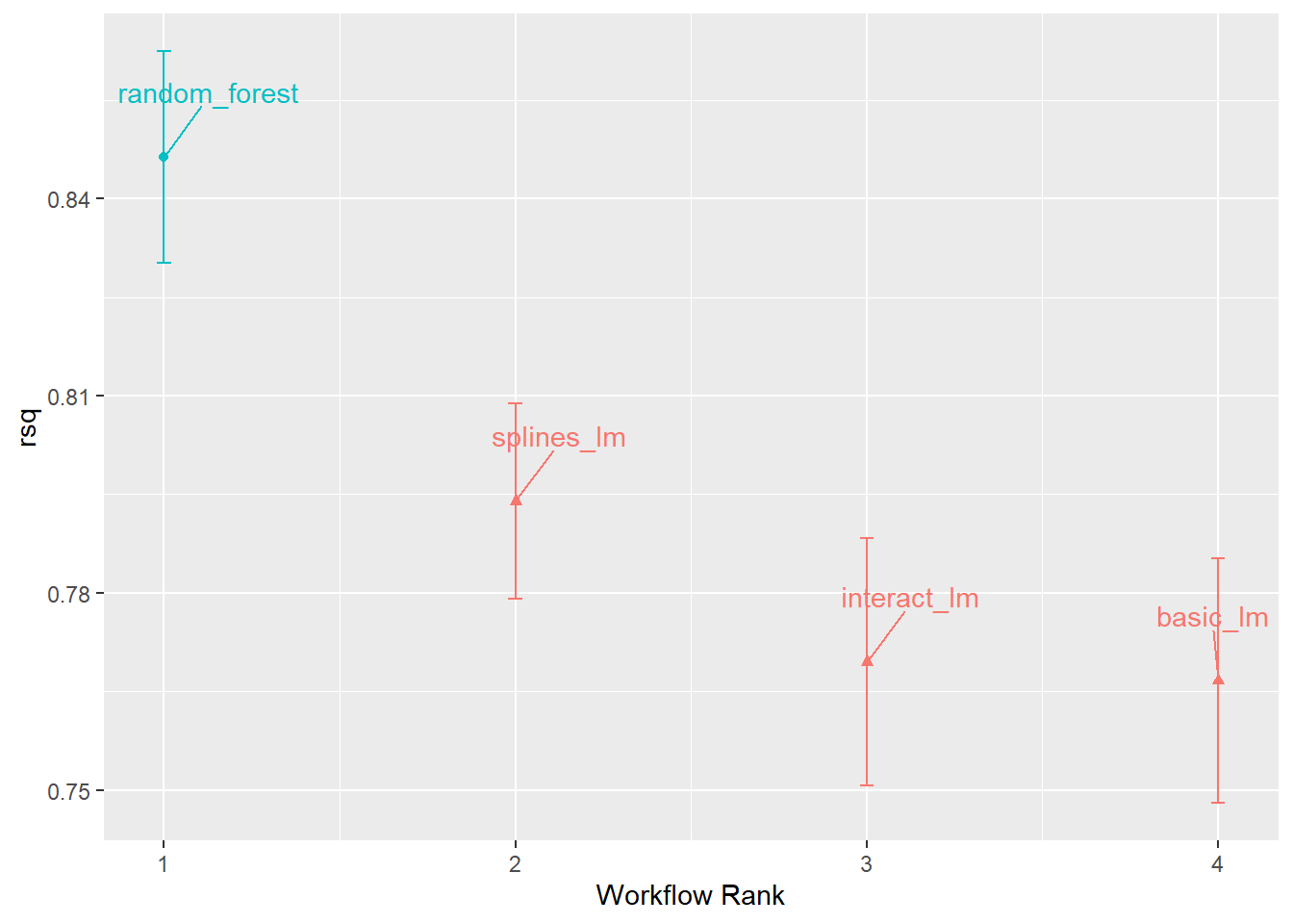
因为每个工作流程用多组分析、评估集合计算了多个\(R^2\)结果, 所以可以做成置信区间的图形。 这里的\(R^2\)定义为因变量和预测值的相关系数的平方。
47.2.2 用再抽样技术计算的模型性能指标的选择
使用不同的性能指标比较各个模型, 最后选出的最优模型可能会不一致。 这就需要我们了解这些性能指标, 然后根据需要选取。
因为不同的模型使用了相同的交叉验证分层数据, 所以这些模型计算得到的同一性能指标的相同交叉验证层之间的值有很强的正相关性。 这样,在用统计检验比较两个模型时, 这种正相关性会干扰模型比较。 比如, 不能用独立两样本检验比较两个模型的\(RMSE\)指标是否相等, 强正相关性会使得两个模型的指标之间的差异变小, 使得检验不出显著差异。
作为显著性检验的替代, 可以预先确定一个“实际效应”阈值, 当差别超过这个阈值时就认为两个模型有差异。 虽然这种做法比较主观, 但是在选择模型时很有用。
47.2.4 用贝叶斯方法比较模型
仍可以用性能指标作为因变量, 建立方差分析模型, 但是假设模型系数、误差标准差有先验分布, 然后计算后验分布。 可以将不同的交叉验证层作为一个随机效应截距。 tidyposterior包可以用来进行这样的贝叶斯计算。
比较4个模型的\(R^2\)的例子:
## Warning: package 'tidyposterior' was built under R version 4.2.3## Warning: package 'rstanarm' was built under R version 4.2.3## Loading required package: Rcpp##
## Attaching package: 'Rcpp'## The following object is masked from 'package:rsample':
##
## populate## This is rstanarm version 2.21.4## - See https://mc-stan.org/rstanarm/articles/priors for changes to default priors!## - Default priors may change, so it's safest to specify priors, even if equivalent to the defaults.## - For execution on a local, multicore CPU with excess RAM we recommend calling## options(mc.cores = parallel::detectCores())rsq_anova <-
perf_mod(
four_models,
metric = "rsq",
prior_intercept = rstanarm::student_t(df = 1),
chains = 4,
iter = 5000,
seed = 1102
)用\(R^2\)的后验分布的随机样本代表后验分布:
## Rows: 40,000
## Columns: 2
## $ model     <chr> "random_forest", "basic_lm", "interact_lm", "splines_lm", "r…
## $ posterior <dbl> 0.8492608, 0.7673806, 0.7805280, 0.7913962, 0.8517934, 0.768…四个模型的\(R^2\)的后验分布图形:
model_post |>
  mutate(model = forcats::fct_inorder(model)) |>
  ggplot(aes(x = posterior)) +
  geom_histogram(
    bins = 50,
    color = "white",
    fill = "blue",
    alpha = 0.4) +
  facet_wrap(~ model, ncol = 1)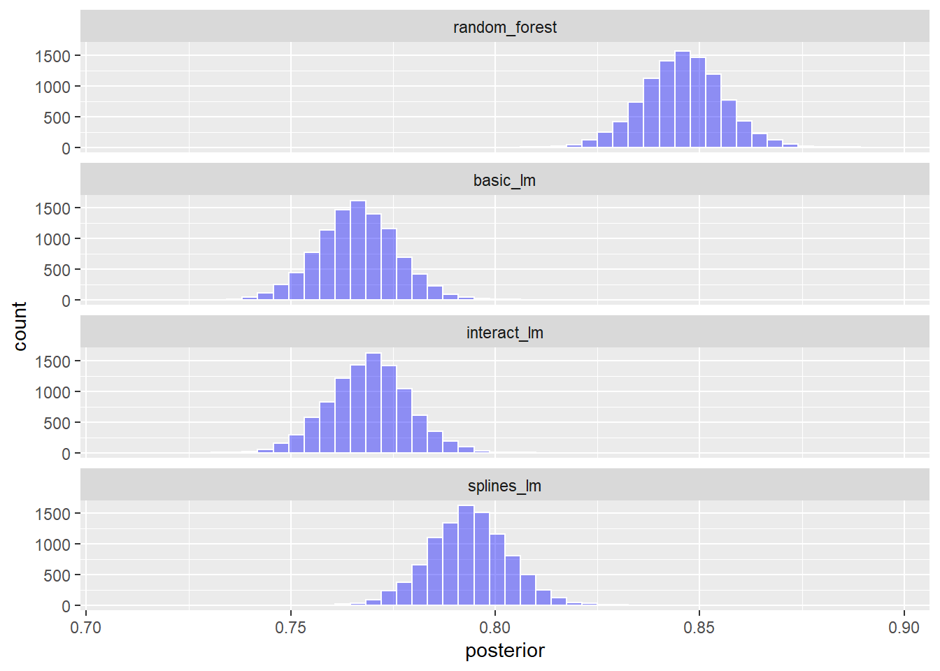
各个模型的\(R^2\)置信区间图形:
library(ggrepel)
autoplot(rsq_anova) +
  geom_text_repel(
    aes(label = workflow),
    nudge_x = 1/8, nudge_y = 1/100) +
  theme(legend.position = "none")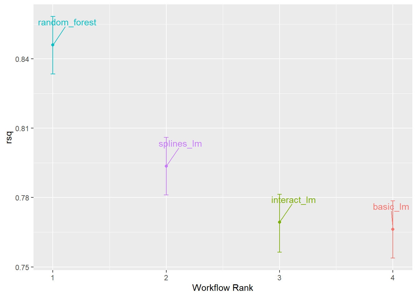
不同模型的后验分布随机样本是按行一一对应的, 所以很容易生成比较用的样本。 例如, 比较基本的线性模型和加入交互项、样条项的线性模型:
rqs_diff <-
  contrast_models(
    rsq_anova,
    list_1 = "splines_lm",
    list_2 = "basic_lm",
    seed = 1104)

rqs_diff |>
  as_tibble() |>
  ggplot(aes(x = difference)) +
  geom_vline(xintercept = 0, lty = 2) +
  geom_histogram(
    bins = 50, color = "white",
    fill = "red", alpha = 0.4)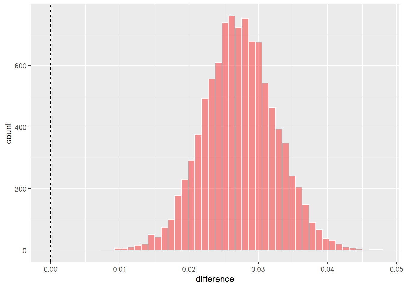
这是`list_1 - list_2\(的\)R^2$后验样本的直方图。
计算差值的可信区间(credible interval):
## # A tibble: 1 × 6
##   contrast               probability   mean  lower  upper  size
##   <chr>                        <dbl>  <dbl>  <dbl>  <dbl> <dbl>
## 1 splines_lm vs basic_lm           1 0.0273 0.0189 0.0359     0
其中的概率是差值大于0的概率。 差值的均值仅有\(0.0085\), 如果要求差值显著超过\(0.02\)才算是有效的差距, 可以如下计算:
## # A tibble: 1 × 4
##   contrast               pract_neg pract_equiv pract_pos
##   <chr>                      <dbl>       <dbl>     <dbl>
## 1 splines_lm vs basic_lm 0 0.0771 0.923其中pract_equiv列是差值的后验样本中位于[-size, size]区间内的比例,
可以认为以\(0.02\)为有效差距阈值,
则两个方法之间没有有效差距。
可以用图形表示多组之间是否有有效差距:
autoplot(
  rsq_anova, type = "ROPE", size = 0.02) +
  geom_text_repel(aes(label = workflow)) +
  theme(legend.position = "none")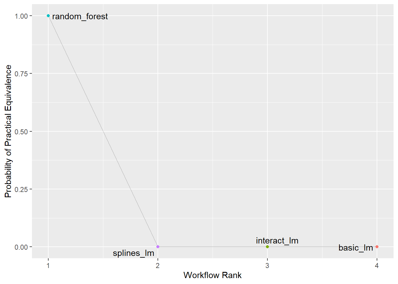
图形说明,以\(0.02\)为有效差值的阈值, 则三个线性模型都和随机森林模型有有效差距, 而这三个之间没有有效差距。
为了提高贝叶斯推断的精度, 可以使用重复交叉验证方法生成更多的交叉验证样本, 这可以缩短贝叶斯可信区间长度。
47.3 模型参数调优和过度拟合问题
47.3.1 概念
在建模时, 有些模型参数是直接从训练数据估计的; 而其它一些参数, 称为调节参数(tuning parameters)或者超参数(hypterparmeters), 不能直接估计而是需要预先指定。
考虑线性回归模型 \[ y_i = a + b x_i + e_i, \ i=1,2,\dots,n . \] 其中的参数\(a, b\)可以用最小二乘估计法直接从训练集得到估计结果。
有一些参数则不能直接从训练集估计,称为“调节参数”或者“超参数”。 比如:
- 随机森林算法在训练集上训练之前, 需要指定树的深度。
- GBM算法需要指定树的棵数、树的深度、学习率。
- lasso回归需要指定\(L^1\)惩罚项的系数, 称为调节参数, 不能直接估计。
- 在多层神经网络模型中, 网络的层数、每一层的节点数、选用的激活函数, 都需要预先确定, 不能从训练集估计。
- 深度神经网络中梯度下降算法的改进版本, 需要确定学习率,动量系数, 运行的轮数(epochs)等, 也需要调优,但不能从训练集估计。
有时需要对预处理步骤调优,如:
- 在主成分分析、偏最小二乘中, 可以对原始变量作变换, 突出其线性相关性; 可以选择输出的降维变量个数。
- 在对缺失值进行插补时, 可以对某一变量用最近邻方法插补, 这时需要确定使用的近邻个数。
有一些统计模型有结构上的不同设置, 这可以看成是模型比较问题, 也可以广义地看成是模型调优问题:
- 对于二值因变量建立广义线性模型, 联系函数一般使用logit函数, 但也可以使用probit或者余重对数(complementary log-log)。
- 在线性混合模型中, 随机效应的方差阵可以指定为常数方差对角阵、 对角阵或者自回归的、Toeplitz的。
不能作为参数调优问题的一个典型例子是贝叶斯分析中的先验分布选择。 先验分布代表了研究者对参数的先验知识, 这不能从训练集中调优, 否则就违背了贝叶斯分析的原则。
另外, 在随机森林算法和bagging算法中, 树的棵数也不需要调优, 只要取得比较大(对随机森林,达到几千,对bagging,50到100即可), 性能就没有进一步的改进, 也不会造成过度拟合问题。
47.3.2 参数调优的标准
为了参数调优应该选用什么样的性能指标? 这依赖于考虑的模型以及建模的目的。 如果主要目的是进行统计推断, 而模型选择或比较可以通过统计推断方法进行, 可以利用统计假设检验、置信区间来进行模型比较, 一般这不需要使用再抽样技术,只用训练集上的检验结果即可; 但是, 如果建模目的是预报, 则预报精度是更重要的考虑, 应使用再抽样技术进行比较, 统计推断得到的模型比较结论与按预报精度得到结论有可能不一致。
47.3.3 超参数选择的问题
超参数在许多模型中控制的是模型的复杂度。 模型过于简单, 则模型对训练集和测试集的预报效果都不好; 模型越复杂, 越能够抓住数据中的复杂规律, 但是也可能产生过度拟合, 即抓住了训练集中一些随机发生的非规律性的模式, 在测试集上表现很差。 见33.6的示例。
在选择超参数时必须使用再抽样技术, 把估计普通参数的数据与选择超参数的数据分开, 否则选择超参数就会倾向于完美拟合训练集, 产生过度拟合, 在测试集上表现会很差。
47.3.4 超参数优化的两种常用策略
超参数优化经常使用网格搜索法(grid search)和迭代法(iterative search)。
网格法有些像是方差分析中的全面试验设计, 每个要优化的超参数选取若干个最可能的值, 然后将这些超参数进行完全组合。 比如, 超参数A取值为\(0.1, 0.2\), 超参数B取值\(2, 5\), 超参数C取值\(10, 100, 1000\), 则网格设计表如下:
| A | B | c |
|---|---|---|
| 0.1 | 2 | 10 |
| 0.1 | 2 | 100 |
| 0.1 | 2 | 1000 |
| 0.1 | 5 | 10 |
| 0.1 | 5 | 100 |
| 0.1 | 5 | 1000 |
| 0.2 | 2 | 10 |
| 0.2 | 2 | 100 |
| 0.2 | 2 | 1000 |
| 0.2 | 5 | 10 |
| 0.2 | 5 | 100 |
| 0.2 | 5 | 1000 |
共有\(2 \times 2 \times 3 = 12\)个网格点, 需要对12种超参数组合用再抽样技术进行比较。
除了使用以上的完全组合作为网格外, 还可以使用不规则的网格, 类似于拟随机数设计, 使得网格点在空间中既分布比较均匀, 又互相远离, 称为“空间填充设计”。
迭代搜索法则从某个初始的参数组合的出发, 针对指定的目标函数(即利用再抽样方法计算的模型性能指标)进行优化迭代, 原则上可以使用任意的优化迭代方法, 但是要注意到目标函数利用了再抽样方法, 所以目标函数值有随机误差, 不能要求太高的优化精度, 一般可以规定搜索使用的时间阈值或者迭代步数阈值。
一种迭代方法是结合了网格法的简单, 与迭代搜索法的灵活性, 即指定一个参数组合的较大网格, 然后在这些网格点上随机地跳跃, 直到达到规定的运行时间或者搜索步数, 使用已搜索到的最优超参数组合作为输出。
还可以用网格法搜索迭代初始值, 然后用网格法得到的参数组合作为初值进行迭代搜索。
47.3.5 调优超参数管理
tidymodels系统用dials扩展包管理超参数组合。 因为tidymodels对同一问题支持多种模型, 对同一模型支持多种计算引擎, 所以将超参数分为两个级别:
- 主要参数, 这是同一模型的每个计算引擎都要设置的, 只不过使用的参数名称不一定相同, parsnip对这些参数进行了统一化, 只要使用parsnip规定的参数名称即可。
- 引擎特有的参数,
这些参数一般不需要进行优化。
如需指定,
可以在
set_engine()函数中与计算引擎一同指定。
例如:
rand_forest(trees = 2000, min_n = 10)  # trees和min_n是主要参数
  set_engine("ranger",
regularization.factor = 0.5) # regularization.factor是引擎特有参数在指定模型的函数(如上面的rand_forest())中,
可以指定超参数的值,
也可以将超参数说明为= tune(),
则是规定该超参数通过超参数调优获得。
如:
tune()函数并不实际运行,
只起到说明作用,
后面要讲到的模型调优函数则能够识别工作流程中的这样的说明,
进行实际的参数调优。
这些参数调优函数能够识别这些要调优的参数,
自动获得其取值范围和常用值。
用extract_parameter_set_dials()可以查看哪些超参数需要调优:
## Collection of 2 parameters for tuning
##
##  identifier  type    object
##        mtry  mtry nparam[?]
##       min_n min_n nparam[+]
##
## Model parameters needing finalization:
##    # Randomly Selected Predictors ('mtry')
##
## See `?dials::finalize` or `?dials::update.parameters` for more information.nparam[?]表示取值范围待定的数值型参数,
它对应的mtry参数是随机森林算法每一次分叉时允许使用的自变量个数,
这个数值依赖于训练数据集中的自变量个数。
params[+]表示要调优的min_n参数是一个数值型参数且范围可确定。
结果中的identifier在有多于一处需要对同一参数调优时可以区分不同的调优参数,
比如,
有两个自变量都需要用ns()函数转换,
则需要有两个自由度参数,
程序如:
ames_rec <-
  recipe(Sale_Price ~ Neighborhood + Gr_Liv_Area
    + Year_Built + Bldg_Type
    + Latitude + Longitude,
    data = ames_train)  |>
  step_log(Gr_Liv_Area, base = 10) |>
  step_other(Neighborhood, threshold = tune()) |>
  step_dummy(all_nominal_predictors()) |>
  step_interact( ~ Gr_Liv_Area:starts_with("Bldg_Type_") ) |>
  step_ns(Longitude, deg_free = tune("longitude df")) |>
  step_ns(Latitude,  deg_free = tune("latitude df"))

recipes_param <- extract_parameter_set_dials(ames_rec)
recipes_param
## Collection of 3 parameters for tuning
##
## identifier type object
## threshold threshold nparam[+]
## longitude df deg_free nparam[+]
## latitude df deg_free nparam[+]其中tune()函数增加了一个用来作为调节参数标识符的输入项。
预处理步骤和模型中都可以有超参数, 将二者结合到工作流程中以后, 这些超参数都可以看到, 如:
wflow_param <-
  workflow() |>
  add_recipe(ames_rec) |>
  add_model(rf_mod) |>
  extract_parameter_set_dials()
wflow_param
## Collection of 5 parameters for tuning
##
## identifier type object
## mtry mtry nparam[?]
## min_n min_n nparam[+]
## threshold threshold nparam[+]
## longitude df deg_free nparam[+]
## latitude df deg_free nparam[+]
##
## Model parameters needing finalization:
## # Randomly Selected Predictors ('mtry')
##
## See `?dials::finalize` or `?dials::update.parameters` for more information.wflow_param这样的对象被超参数调优函数使用。
查看某一个超参数的设置:
## Threshold (quantitative)
## Range: [0, 0.1]可以修改wflow_param这样的对象,
如:
wflow_param <- wflow_param |>
update(threshold = threshold(c(0.8, 1.0)))
wflow_param |>
  extract_parameter_dials("threshold")
## Threshold (quantitative)
## Range: [0.8, 1]又如,
人为确定mtry参数的取值范围:
wflow_param <- wflow_param |>
  update(mtry = mtry(c(1, 70)))
wflow_param |>
  extract_parameter_dials("mtry")
## # Randomly Selected Predictors (quantitative)
## Range: [1, 70]注意ames数据集共有74个变量,
最多可以有73个自变量。
但是,如果预处理步骤或者算法可能会增删自变量,
这样的范围指定有可能不适合,
可以对调优参数对象使用finalize()函数,
指定一个训练集获得实际可用的参数范围,如:
pca_rec <-
  recipe(Sale_Price ~ ., data = ames_train) |>
  # 将与面积有关的自变量用主成分分析法压缩:
  step_normalize(contains("SF")) |>
  # 用方差累计贡献率选择主成分个数
  step_pca(contains("SF"), threshold = .95)

updated_param <-
  workflow() |>
  add_model(rf_mod) |>
  add_recipe(pca_rec) |>
  extract_parameter_set_dials() |>
  # 这一步可以确定mtry的范围:
  finalize(ames_train |> select(-Sale_Price))
updated_param
## Collection of 2 parameters for tuning
##
## identifier type object
## mtry mtry nparam[+]
## min_n min_n nparam[+]## # Randomly Selected Predictors (quantitative)
## Range: [1, 73]引擎特有的超参数也可以用extract_parameter_set_dials()管理。
有些超参数使用变换后的值更方便,
需要了解这些变换,
人为指定范围时也要使用变换后的范围,
如:
## Amount of Regularization (quantitative)
## Transformer: log-10 [1e-100, Inf]
## Range (transformed scale): [-10, 0]
这个参数使用时用了实际参数值的常用对数变换,
指定范围时需要在变换后指定。
比如,
指定penalty在\([0.1, 1]\)范围,
需要作常用对数变换,
指定范围为\([-1, 0]\),
如:
##    Min. 1st Qu.  Median    Mean 3rd Qu.    Max.
## 0.1000 0.1797 0.3193 0.3897 0.5710 0.9926上例指定了penalty在\([0.1, 1]\)范围,
并随机生成了1000个值,
计算这些值的简单统计量(在没有对数变换的基础上计算)。
可以用trans = NULL指定在未变换的基础上指定范围,
如:
## Amount of Regularization (quantitative)
## Range: [0.1, 1]
47.4 超参数调优的网格搜索法
网格搜索法预先确定要试验的超参数组合, 并对这些组合逐一使用再抽样技术计算模型性能参数, 从而找到最优超参数组合。
47.4.1 规则网格与不规则网格
规则网格法产生的超参数网格类似于方差分析中的完全试验设计, 由每个超参数选择少量水平值作完全组合产生网格。 非规则网格则是在超参数组合空间内直接布点。
以单隐藏层神经网络为例。 要调节的超参数包括隐藏层单元数、拟合迭代的轮数(epochs)、权重衰减系数。
指定模型、引擎,
在模型函数mlp()中指定主要超参数,
三个主要超参数都需要调优:
mlp_spec <-
  mlp(
    hidden_units = tune(),
    penalty = tune(),
    epochs = tune()) |>
  set_engine("nnet", trace = 0) |>
set_mode("classification")用extract_parameter_set_dials()提取超参数集合:
用extract_parameter_dials()显示各个超参数设置:
## # Hidden Units (quantitative)
## Range: [1, 10]## Amount of Regularization (quantitative)
## Transformer: log-10 [1e-100, Inf]
## Range (transformed scale): [-10, 0]## # Epochs (quantitative)
## Range: [10, 1000]47.4.1.1 使用规则网格
前面的mlp_param仅是列出了要调优的参数以及每个参数的可取范围,
但是没有给出具体的参数组合。
规则网格法则对每个超参数指定若干个典型取值,
然后完全组合。
tidyr包的crossing()函数可以生成这样的完全组合,
如:
## # A tibble: 12 × 3
##    hidden_units penalty epochs
##           <int>   <dbl>  <dbl>
##  1            1     0      100
##  2            1     0      200
##  3            1     0.1    100
##  4            1     0.1    200
##  5            2     0      100
##  6            2     0      200
##  7            2     0.1    100
##  8            2     0.1    200
##  9            3     0      100
## 10            3     0      200
## 11            3     0.1    100
## 12            3     0.1    200
实际上, dials包的调优函数给出的超参数设置可以自动产生规则网格, 所以仅在用户有经验时才人为指定规则网格, 如:
## # A tibble: 8 × 3
##   hidden_units      penalty epochs
##          <int>        <dbl>  <int>
## 1            1 0.0000000001     10
## 2           10 0.0000000001     10
## 3            1 1                10
## 4           10 1                10
## 5            1 0.0000000001   1000
## 6           10 0.0000000001   1000
## 7            1 1              1000
## 8 10 1 1000其中的levels输入指定每个超参数要取几个典型水平值。
也可以每个超参数分别指定水平值个数,如:
## # A tibble: 12 × 3
##    hidden_units      penalty epochs
##           <int>        <dbl>  <int>
##  1            1 0.0000000001     10
##  2            5 0.0000000001     10
##  3           10 0.0000000001     10
##  4            1 1                10
##  5            5 1                10
##  6           10 1                10
##  7            1 0.0000000001   1000
##  8            5 0.0000000001   1000
##  9           10 0.0000000001   1000
## 10            1 1              1000
## 11            5 1              1000
## 12           10 1              1000
也可以不进行完全试验, 而是在上述的完全组合中选一部分, 比如正交设计法。
当超参数个数较多时, 对大多数模型来说规则网格法耗时较多, 也有一些模型例外。 规则网格法优点是每个超参数的调优作用比较容易理解, 需要的话也可以研究一些交互作用效应。
47.4.1.2 非规则网格法
最简单的非规则网格方法是在超参数取值范围内进行随机抽样。
这样理论上可以比较均匀,
但是结果具有随机性,
实际上可能有些点距离较近,
而有些参数空间位置附近没有网格点。
用grid_random()产生这样的网格。
如:
##   hidden_units       penalty              epochs
##  Min.   : 1.000   Min.   :0.0000000   Min.   : 10.0
##  1st Qu.: 3.000   1st Qu.:0.0000000   1st Qu.:265.8
##  Median : 5.000   Median :0.0000061   Median :497.0
##  Mean   : 5.381   Mean   :0.0437435   Mean   :509.5
##  3rd Qu.: 8.000   3rd Qu.:0.0026854   3rd Qu.:761.0
## Max. :10.000 Max. :0.9814405 Max. :999.0其中的size是非规则网格点个数。
如果某些超参数进行了变换,
随机抽样是在变换后的范围内均匀抽样的。
更合理的做法是用“空间填充设计”, 其目标是尽可能覆盖整个超参数空间范围, 又避免相距过近的点。 具体方法有拉丁方设计, 最大熵设计, 最大投影设计, 等等。
dials包能使用拉丁方设计与最大熵设计。 使用拉丁方设计如:
library(ggforce)
set.seed(1303)
mlp_param |>
  grid_latin_hypercube(
    size = 20, original = FALSE) |>
  ggplot(aes(x = .panel_x, y = .panel_y)) +
  geom_point() +
  geom_blank() +
  facet_matrix(
    vars(hidden_units, penalty, epochs),
      layer.diag = 2) +
  labs(title = "Latin Hypercube design with 20 candidates")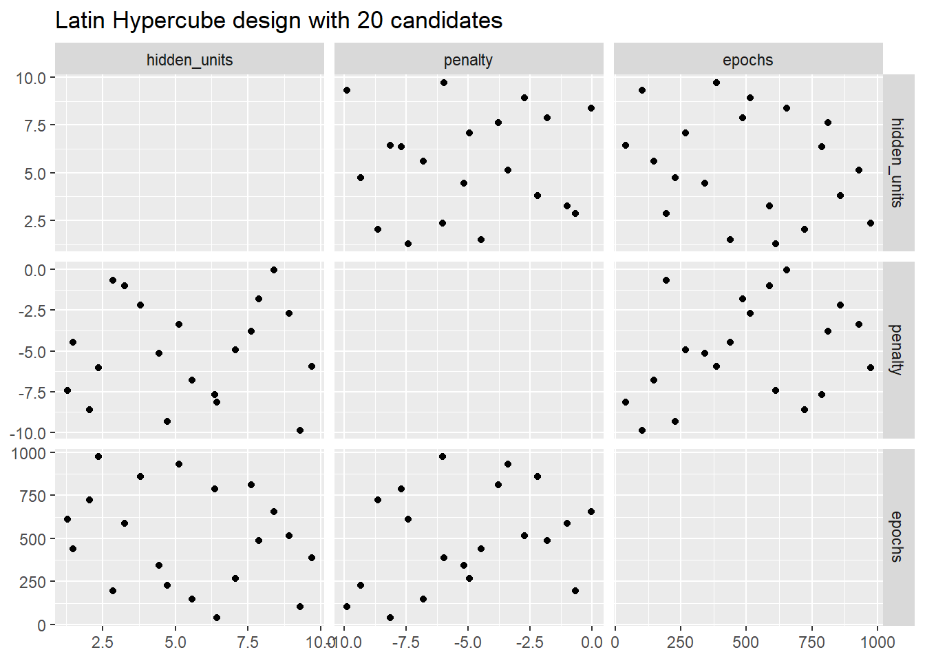
tune扩展包默认使用最大熵设计产生非规则网格,
函数为grid_max_entropy()
这种方法覆盖超参数空间效果好,
能更快搜索最优超参数组合。
47.4.2 评估不同超参数组合的性能
使用网格搜索法寻找最优超参数组合, 本质上是对每一超参数组合利用重抽样方法计算模型性能指标。
以modeldata包的cells数据集作为示例。
数据集中有2019例肺癌病人的医学影像数据,
因变量class取两个类别值,
56个自变量则是细胞不同部位的大小、形状、密度测量值,
自变量存在较高相关性,
自变量分布有的不对称。
建模目的是预测分类。
上面删去的变量case用来区分每个病例,
既不是因变量也不是自变量。
本节仅演示参数调优问题, 所以不进行训练集、测试集拆分, 使用所有观测作为训练集。 使用十折交叉验证进行参数调优:
因为自变量的自相关性,
预处理增加一个用主成分分析降维的步骤,
保留主成分个数也作为预处理步骤的待调优超参数。
因为有些自变量分布不对称,
这使得基于方差的主成分方法受到离群值的影响较大,
所以利用了step_YeoJohnson()将自变量分布变得更加对称。
因为获得的主成分的方差是递减的,
所以在产生主成分以后再次用step_normalize()进行变量标准化。
程序如下:
mlp_rec <-
  recipe(class ~ ., data = cells) |>
  step_YeoJohnson(all_numeric_predictors()) |>
  step_normalize(all_numeric_predictors()) |>
  step_pca(
    all_numeric_predictors(),
    num_comp = tune()) |>
  step_normalize(all_numeric_predictors())

mlp_spec <-
  mlp(
    hidden_units = tune(),
    penalty = tune(),
    epochs = tune()) |>
  set_engine("nnet", trace = 0) |>
  set_mode("classification")

mlp_wflow <-
  workflow() |>
  add_model(mlp_spec) |>
add_recipe(mlp_rec)下面提取用tune()指定的待调优超参数集合,
并人为修改部分超参数的可选范围:
mlp_param <-
  mlp_wflow |>
  extract_parameter_set_dials() |>
  update(
    epochs = epochs(c(50, 200)),
    num_comp = num_comp(c(0, 40))
)其中的num_comp是PCA预处理步的保留主成分个数。
在step_pca()中,
如果主成分个数选取为0个,
就作为使用原始变量而不进行维数压缩的处理。
下面利用tune_grid()函数在已经定义的超参数网格上进行超参数调优。
这与fit_resamples()本质上相同,
但对多组超参数组合进行计算。
tune_grid()以工作流程和一个再抽样对象(如交叉验证对象)为输入。
可以指定要计算的性能指标集合。
最好利用并行计算功能。 程序如:
library(doParallel)

# 产生一个集群对象并注册
cl <- makePSOCKcluster(8)
registerDoParallel(cl)

roc_res <- metric_set(roc_auc) # 性能指标集合

set.seed(1305)
mlp_reg_tune <-
  mlp_wflow |>
  tune_grid(
    cell_folds,
    grid = mlp_param |> grid_regular(levels = 3),
    metrics = roc_res )

# 取消集群对象
stopCluster(cl)

# 卸载并行库
detach("package:doParallel")

mlp_reg_tune
## # Tuning results
## # 10-fold cross-validation
## # A tibble: 10 × 4
## splits id .metrics .notes
## <list> <chr> <list> <list>
## 1 <split [1817/202]> Fold01 <tibble [81 × 8]> <tibble [0 × 3]>
## 2 <split [1817/202]> Fold02 <tibble [81 × 8]> <tibble [0 × 3]>
## 3 <split [1817/202]> Fold03 <tibble [81 × 8]> <tibble [0 × 3]>
## 4 <split [1817/202]> Fold04 <tibble [81 × 8]> <tibble [0 × 3]>
## 5 <split [1817/202]> Fold05 <tibble [81 × 8]> <tibble [0 × 3]>
## 6 <split [1817/202]> Fold06 <tibble [81 × 8]> <tibble [0 × 3]>
## 7 <split [1817/202]> Fold07 <tibble [81 × 8]> <tibble [0 × 3]>
## 8 <split [1817/202]> Fold08 <tibble [81 × 8]> <tibble [0 × 3]>
## 9 <split [1817/202]> Fold09 <tibble [81 × 8]> <tibble [0 × 3]>
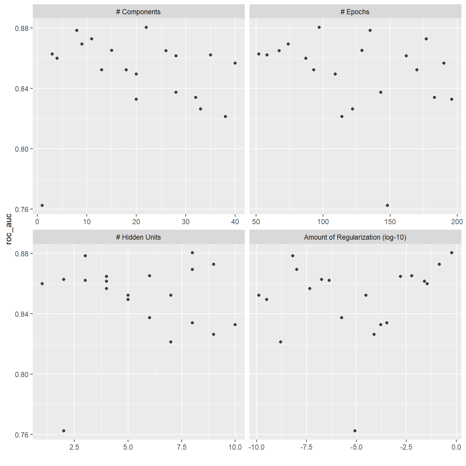
## 10 <split [1818/201]> Fold10 <tibble [81 × 8]> <tibble [0 × 3]>共有4个调优超参数, 对于规则网格, 试验设计类似完全试验设计, 可以作图显示不同参数的性能比较:
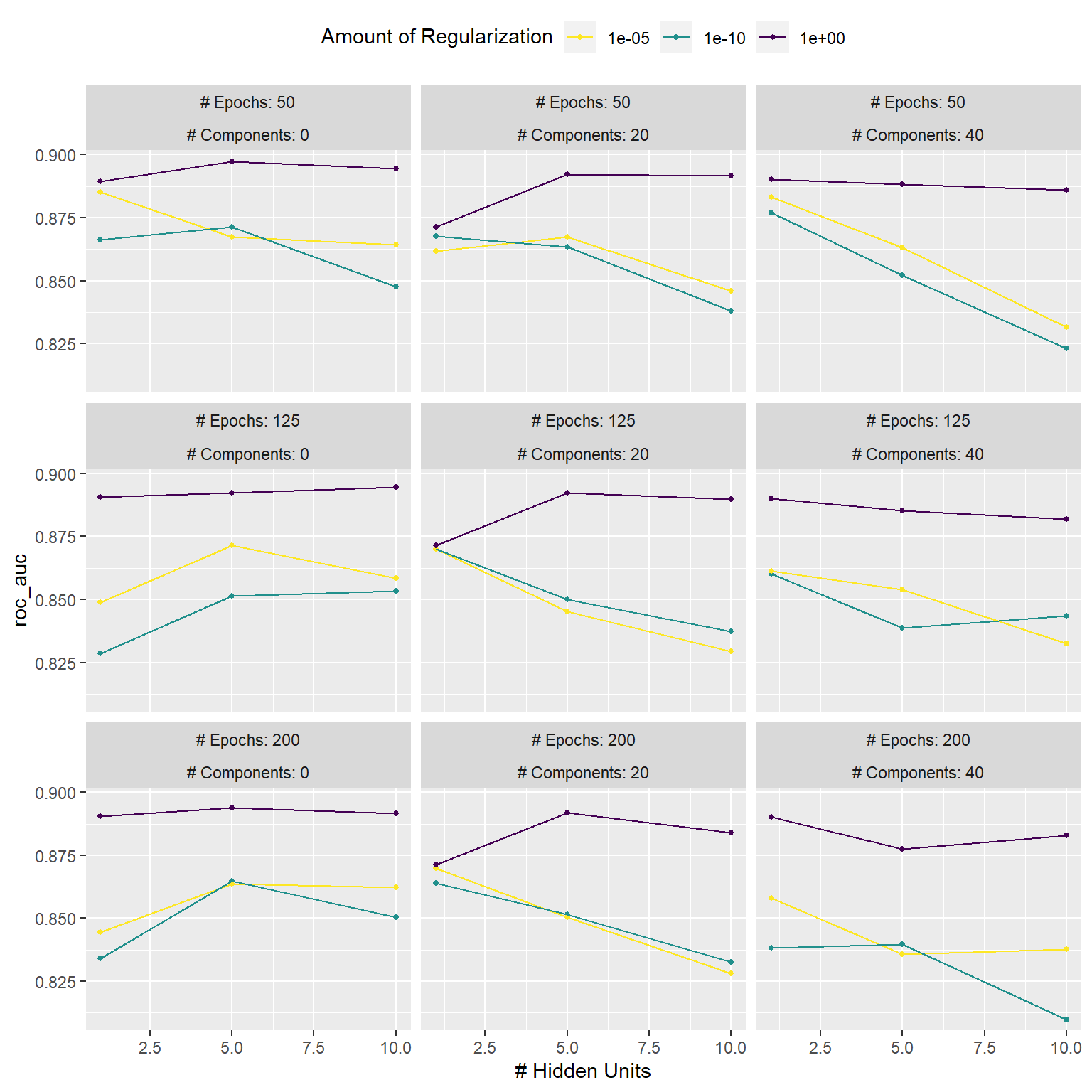
从图形明显看出, 超参数“正则性惩罚的量”以最高值1为最优。 epochs的差异不明显。 主成分个数好像以0个(不作主成分变换)为优。 隐藏单元的个数的影响与其它超参数有交互作用, 且仅在正则性惩罚非最优时影响较大。
用show_best()可以从tune_grid()的输出结果中显示若干个性能相近的最优模型:
| hidden_units | penalty | epochs | num_comp | .metric | mean | n | std_err | .config |
|---|---|---|---|---|---|---|---|---|
| 5 | 1 | 50 | 0 | roc_auc | 0.8973350 | 10 | 0.0085720 | Preprocessor1_Model08 |
| 10 | 1 | 125 | 0 | roc_auc | 0.8945163 | 10 | 0.0089850 | Preprocessor1_Model18 |
| 10 | 1 | 50 | 0 | roc_auc | 0.8944248 | 10 | 0.0096021 | Preprocessor1_Model09 |
| 5 | 1 | 200 | 0 | roc_auc | 0.8938910 | 10 | 0.0078434 | Preprocessor1_Model26 |
| 5 | 1 | 125 | 0 | roc_auc | 0.8924622 | 10 | 0.0082247 | Preprocessor1_Model17 |
仍使用结果表格中的mean列作为不同超参数组合的评价指标。
从结果看,
有必要增加penalty超参数的值进行网格搜索。
为了使用空间填充设计的非规则网格搜索法,
可以在tune_grid()中指定grid =一个网格点个数,
或者取为grid_max_entropy()这样的网格生成函数结果。
如:
roc_res <- metric_set(roc_auc) # 性能指标集合

set.seed(1306)
mlp_sfd_tune <-
  mlp_wflow |>
  tune_grid(
    cell_folds,
    grid = 20,
    param_info = mlp_param, # 指定调整过范围的超参数集合
    metrics = roc_res
  )
mlp_sfd_tune
## # Tuning results
## # 10-fold cross-validation
## # A tibble: 10 × 4
## splits id .metrics .notes
## <list> <chr> <list> <list>
## 1 <split [1817/202]> Fold01 <tibble [20 × 8]> <tibble [0 × 3]>
## 2 <split [1817/202]> Fold02 <tibble [20 × 8]> <tibble [0 × 3]>
## 3 <split [1817/202]> Fold03 <tibble [20 × 8]> <tibble [0 × 3]>
## 4 <split [1817/202]> Fold04 <tibble [20 × 8]> <tibble [0 × 3]>
## 5 <split [1817/202]> Fold05 <tibble [20 × 8]> <tibble [0 × 3]>
## 6 <split [1817/202]> Fold06 <tibble [20 × 8]> <tibble [0 × 3]>
## 7 <split [1817/202]> Fold07 <tibble [20 × 8]> <tibble [0 × 3]>
## 8 <split [1817/202]> Fold08 <tibble [20 × 8]> <tibble [0 × 3]>
## 9 <split [1817/202]> Fold09 <tibble [20 × 8]> <tibble [0 × 3]>
## 10 <split [1818/201]> Fold10 <tibble [20 × 8]> <tibble [0 × 3]>对非规则网络的调优结果,
用autoplot()作图,
类似于假设了一个可加模型,
作因变量(性能指标)对各个自变量的散点图:
因为实际上超参数之间可能有交互作用, 所以上述的图形可能不完全反映超参数组合的影响。
用show_best()显示最优的几个网格点:
## # A tibble: 5 × 9
##   hidden_units       penalty epochs num_comp .metric  mean     n std_err .config
##          <int>         <dbl>  <int>    <int> <chr>   <dbl> <int>   <dbl> <chr>
## 1            8 0.594             97       22 roc_auc 0.880    10 0.00998 Prepro…
## 2            3 0.00000000649    135        8 roc_auc 0.878    10 0.00955 Prepro…
## 3            9 0.141            177       11 roc_auc 0.873    10 0.0104  Prepro…
## 4            8 0.0000000103      74        9 roc_auc 0.869    10 0.00761 Prepro…
## 5 6 0.00581 129 15 roc_auc 0.865 10 0.00658 Prepro…其中最优的AUC值\(0.88\), 比规则网格达到的\(0.89\)略差。 规则网格计算了81个网格点, 这里仅使用了20个网格点。
在用网格法进行参数调优时, 还应该考虑多个性能指标, 而不是完全按照同一个性能指标。 另外, 还可以不选择搜索到的性能指标最优的组合, 而是选用次优但是更简单的组合。 是否“更简单”可以用代表模型复杂度的参数来衡量。
参数调优仅为了搜索最优的超参数组合,
所以在tune_grid()运行完以后一般不需要保存评估集上的因变量预测值和各个分析、评估集上计算的性能指标,
如果需要可以用control参数输入函数control_grid()的设置结果。
在control_grid()中设置extract = TRUE可以保留预处理、拟合参数结果,
设置save_pred = TRUE可以保留预测值,
在调优后用collect_predictions()提取预测值。
47.4.3 确定最优超参数
tune_grid()函数仅在网格点上计算模型性能指标,
show_best()函数可以显示最优的若干组超参数组合,
但都用来不在训练集上估计模型,
所以为了确定某个参数组合用来估计模型,
可以人为记录超参数组合然后直接在建模函数值指定超参数值,
还可以用select_*()函数从tune_grid()结果中挑选超参数组合。
例如,select_best()取出指定的性能指标最优的超参数组合:
## # A tibble: 1 × 5
##   hidden_units penalty epochs num_comp .config
##          <int>   <dbl>  <int>    <int> <chr>
## 1            5       1     50        0 Preprocessor1_Model08
这用一个单行数据框形式返回了AUC参数最优的超参数组合。
也可以人为输入超参数组合到一个单行的数据框。
得到单行数据框形式的超参数组合后,
用finalize_workflow()函数进行模型估计:
logistic_param <- tibble(
    num_comp = 0, # 主成分个数
    epochs = 125, # 训练轮数
    hidden_units = 1, # 隐藏单元个数
    penalty = 1   # 正则性惩罚项因子
  )

final_mlp_wflow <-
  mlp_wflow |>
  finalize_workflow(logistic_param)
final_mlp_wflow
## ══ Workflow ════════════════════════════════════════════════════════════════════
## Preprocessor: Recipe
## Model: mlp()
##
## ── Preprocessor ────────────────────────────────────────────────────────────────
## 4 Recipe Steps
##
## • step_YeoJohnson()
## • step_normalize()
## • step_pca()
## • step_normalize()
##
## ── Model ───────────────────────────────────────────────────────────────────────
## Single Layer Neural Network Model Specification (classification)
##
## Main Arguments:
## hidden_units = 1
## penalty = 1
## epochs = 125
##
## Engine-Specific Arguments:
## trace = 0
##
## Computational engine: nnet注意上面是超参数固定的工作流程, 还没有进行模型拟合。 在训练集(现在是整个数据集)拟合模型:
如果没有使用工作流程,
而是使用了模型,
则可以使用finalize_model()在模型中固定超参数值。
如果使用了食谱,
可以用finalize_recipe()在食谱中固定预处理超参数值。
47.4.4 调优工作的辅助设置参数工具
usemodels包可以用数据框和模型公式作为输入, 产生模型调优需要的R代码, 所以是一种元编程工具。
例如, 对ames数据集产生xgboost建模用的代码:
## Warning: package 'usemodels' was built under R version 4.2.3use_xgboost(
Sale_Price ~ Neighborhood + Gr_Liv_Area
+ Year_Built + Bldg_Type
+ Latitude + Longitude,
data = ames_train,
# verbose选项指示增加说明生成的代码的注释
verbose = TRUE)## xgboost_recipe <-
## recipe(formula = Sale_Price ~ Neighborhood + Gr_Liv_Area + Year_Built + Bldg_Type +
## Latitude + Longitude, data = ames_train) %>%
## step_zv(all_predictors())
##
## xgboost_spec <-
## boost_tree(trees = tune(), min_n = tune(), tree_depth = tune(), learn_rate = tune(),
## loss_reduction = tune(), sample_size = tune()) %>%
## set_mode("classification") %>%
## set_engine("xgboost")
##
## xgboost_workflow <-
## workflow() %>%
## add_recipe(xgboost_recipe) %>%
## add_model(xgboost_spec)
##
## set.seed(60916)
## xgboost_tune <-
## tune_grid(xgboost_workflow, resamples = stop("add your rsample object"), grid = stop("add number of candidate points"))在生成的代码的食谱部分,
step_novel()对每个分类自变量指定一个训练集中未出现的新水平。
step_dummy()将所有分类自变量转换为哑变量,
且哑变量个数等于类水平数。
step_zv()删去取常数值的自变量。
最后的tune_grid()调用是一个模板,
不能直接运行,
需要将resamples参数设置为某个再抽样分析、评估集对集合,
将grid参数设置为某个规则或非规则超参数网格。
如果在use_xgboost()调用中设置tune = FALSE,
则会生成模型拟合用的R代码,
而不是超参数调优用的R代码。
47.4.5 网格搜索加速工具
参数调优总是比较耗时的, 这里介绍一些加速网格搜索法参数调优的辅助工具。
47.4.5.1 优化子模型
有些模型可以一次拟合就获得多个调优参数对应的性能指标, lasso回归的调节参数就可以这样调优。
偏最小二乘也有这样的特点。 偏最小二乘与主成分分析类似, 但有因变量存在, 在最大化自变量线性组合的方差的同时, 使得因变量与自变量线性组合的相关性达到最大。 一个超参数是要保留的自变量线性组合个数, 一次拟合可以产生保留个数为任意值时的预测结果。
许多常用模型有这样的性质,如:
- 提升方法,可以对不同迭代次数一次性输出对应的预测值。
- 正则化方法,如glmnet包的lasso等功能, 可以对不同惩罚系数值一次性输出对应的预测值。
- 多元适应回归样条(MARS, multivariate adaptive regression splines), 调节参数是要保留的项数, 这可以一次拟合对不同的项数同时输出相应的预测值。
tune扩展包在参数调优时, 会自动利用这些技术。
比如, 使用C5.0作为基础算法的提升法, 将迭代次数作为唯一调优参数时, 可以一次拟合就得到所有迭代次数对应的预测值:
c5_spec <-
  boost_tree(trees = tune()) |>
  set_engine("C5.0") |>
  set_mode("classification")

set.seed(1307)
c5_spec |>
  tune_grid(
    class ~ .,
    resamples = cell_folds,
    grid = data.frame(trees = 1:100),
    metrics = roc_res )
## Warning: package 'C50' was built under R version 4.2.3## # Tuning results
## # 10-fold cross-validation
## # A tibble: 10 × 4
## splits id .metrics .notes
## <list> <chr> <list> <list>
## 1 <split [1817/202]> Fold01 <tibble [100 × 5]> <tibble [0 × 3]>
## 2 <split [1817/202]> Fold02 <tibble [100 × 5]> <tibble [0 × 3]>
## 3 <split [1817/202]> Fold03 <tibble [100 × 5]> <tibble [0 × 3]>
## 4 <split [1817/202]> Fold04 <tibble [100 × 5]> <tibble [0 × 3]>
## 5 <split [1817/202]> Fold05 <tibble [100 × 5]> <tibble [0 × 3]>
## 6 <split [1817/202]> Fold06 <tibble [100 × 5]> <tibble [0 × 3]>
## 7 <split [1817/202]> Fold07 <tibble [100 × 5]> <tibble [0 × 3]>
## 8 <split [1817/202]> Fold08 <tibble [100 × 5]> <tibble [0 × 3]>
## 9 <split [1817/202]> Fold09 <tibble [100 × 5]> <tibble [0 × 3]>
## 10 <split [1818/201]> Fold10 <tibble [100 × 5]> <tibble [0 × 3]>47.4.5.2 利用并行计算功能
tidymodels不自动利用并行计算功能, 而是需要在程序中指定并注册计算集群, 见47.1.4。
进行参数调优过程可以看成如下的两层循环:
# 外层循环,针对不同的分析、评估集对
for(rs in resamples){
  # 提取分析、评估集对
  # 进行预处理

  # 内层循环,针对不同的超参数组合网格点
  for(mod in configarations) {
    # 在分析集上用mod超参数组合估计模型
    # 在评估集上预测,并计算性能指标
  }
}
注意针对超参数组合网格点的循环是在内层循环而不是外层循环。
tune_grid()在并行计算时,
默认仅对外层循环并行化;
可以在tune_grid()中设置参数parallel_over = "everything",
则可以对外层、内层循环的组合进行并行计算。
在预处理计算量不大时,
选用此选项可以充分利用并行计算节点数目,
比仅在外层循环并行化略有改进。
并行计算时要避免使用全局变量,
因为工人节点可能无法访问主控节点的全局变量值。
rlang扩展包的!!运算符可以在设置工作流程参数时将全局变量的值插入到函数调用中。
47.4.5.3 赛跑方法
网格点需要将所有的网格点和所有的分析、评估集对都计算完成, 才能评估不同超参数组合的性能。 如果能在中间就排除某些一定会表现不佳的模型, 就可以加速搜索过程。 在机器学习中这种方法称为“赛跑方法”。 可以不是对所有的分析、评估集对都进行计算, 而是先选一小部分分析、评估集对, 在这样的子集上比较所有的参数组合, 预先将表现特别差的组合删去, 然后再完成其它的分析、评估集对的计算。
程序示例:
library(finetune)

set.seed(1308)
mlp_sfd_race <-
  mlp_wflow |>
  tune_race_anova(
    cell_folds,
    grid = 20,
    param_info = mlp_param,
    metrics = roc_res,
    control = control_race(
      verbose_elim = TRUE)
  )
show_best(mlp_sfd_race, n = 10)
#> # A tibble: 2 × 10
#>   hidden_units penalty epochs num_comp .metric .estimator  mean     n std_err
#>          <int>   <dbl>  <int>    <int> <chr>   <chr>      <dbl> <int>   <dbl>
#> 1            8  0.814     177       15 roc_auc binary     0.887    10 0.0103
#> 2            3  0.0402    151       10 roc_auc binary     0.885    10 0.00810
#> # ℹ 1 more variable: .config <chr>
调优结果仅能显示没有被中途删除的最优组合。
47.5 超参数调优的迭代搜索法
当超参数个数较多时, 网格法需要大量的格子点, 否则在超参数空间中的布点就过于稀疏, 无法抓住最优点。 这时, 可以考虑迭代搜索法。 迭代搜索法的缺点是不一定找到全局近似最优。
各种优化算法都可以使用, 这一节仅介绍贝叶斯优化和模拟退火优化。 以支持向量机建模为例。
47.5.1 支持向量机
使用cells数据集, 使用径向基函数, 要调优的超参数是损失值和径向基的尺度参数\(\sigma\)。
径向基使用点积(向量内积), 所以应该将自变量标准化。 还可以使用PCA方法压缩自变量维数, 这里为了将超参数个数控制为2个就没有使用PCA。
针对cells数据集建立食谱、SVM模型、工作流程:
svm_rec <-
  recipe(class ~ ., data = cells) |>
  # 将自变量分布变得较为对称
  step_YeoJohnson(all_numeric_predictors()) |>
  step_normalize(all_numeric_predictors())

svm_spec <-
  # SVM,基于径向基(radial basis function)
  svm_rbf(cost = tune(), rbf_sigma = tune()) |>
  set_engine("kernlab") |>
  set_mode("classification")

svm_wflow <-
  workflow() |>
  add_model(svm_spec) |>
  add_recipe(svm_rec)
生成交叉验证集:
查看两个超参数的取值范围:
## Cost (quantitative)
## Transformer: log-2 [1e-100, Inf]
## Range (transformed scale): [-10, 5]## Radial Basis Function sigma (quantitative)
## Transformer: log-10 [1e-100, Inf]
## Range (transformed scale): [-10, 0]微调\(\sigma\)的范围:
svm_param <-
  svm_wflow |>
  extract_parameter_set_dials() |>
  update(
    rbf_sigma = rbf_sigma(c(-7, -1)))
后面的两个算法需要一些搜索点的性能指标已知, 所以先构建一个小的网格搜索:
roc_res <- metric_set(roc_auc) # 性能指标集合

set.seed(1401)
start_grid <-
  svm_param |>
  update(
    cost = cost(c(-6, 1)),
    rbf_sigma = rbf_sigma(c(-6, -4))
  ) |>
  grid_regular(levels = 2)

set.seed(1402)
svm_initial <-
  svm_wflow |>
  tune_grid(
    resamples = cell_folds,
    grid = start_grid,
    metrics = roc_res)

collect_metrics(svm_initial)
## # A tibble: 4 × 8
## cost rbf_sigma .metric .estimator mean n std_err .config
## <dbl> <dbl> <chr> <chr> <dbl> <int> <dbl> <chr>
## 1 0.0156 0.000001 roc_auc binary 0.864 10 0.00864 Preprocessor1_Model1
## 2 2 0.000001 roc_auc binary 0.863 10 0.00867 Preprocessor1_Model2
## 3 0.0156 0.0001 roc_auc binary 0.863 10 0.00862 Preprocessor1_Model3
## 4 2 0.0001 roc_auc binary 0.866 10 0.00855 Preprocessor1_Model4网格点上的AUC值(mean列)差别不大,
将作为迭代法的初值。
47.5.2 贝叶斯优化
贝叶斯优化基于已经计算过的超参数组合上的目标函数值(性能指标), 计算出下一个要尝试的超参数组合并用再抽样技术计算其性能指标, 如此进行直到达到最大迭代次数或者不再有改进为止。
贝叶斯优化方法依赖于目标函数的模型与下一个尝试点的推荐算法。
47.5.2.1 高斯过程模型
高斯过程假设所有的观测值服从多元正态分布。 可以用均值函数和协方差函数描述联合分布。 协方差函数的常用模型为 \[ \text{Cov}(y_i, y_j) = \exp\left( -\frac{1}{2} | \boldsymbol x_i - \boldsymbol x_j |^2 \right) + \sigma_{ij}^2 . \] 这个模型意味着, 当超参数(\(\boldsymbol x_i\))组合距离增加时, 对应的性能指标的协方差以负指数速度衰减。 \(\sigma_{ii}=0\)。
使用这样一个概率模型的好处是, 对未来的\(\boldsymbol x_{n+1}\)上的\(y_{n+1}\)的预测, 可以是预测其高斯分布, 用均值和方差限定, 而不是仅有点预测或者区间预测。
对于本例, 已经有\(n=4\)个初始观测, 于是可以拟合高斯过程模型, 预测给出第5个点, 计算其性能指标, 重新拟合高斯过程模型, 预测给出第6个点, 如此重复。
47.5.2.2 购置函数
在估计了高斯过程模型以后, 如何产生推荐的下一个超参数组合点? 可以在一个较大网格超参数上预测对应的性能指标的均值和方差, 并按某种方法在均值大和方差小之间权衡, 给出下一个点的推荐值。 用来权衡的函数称为购置函数。 在均值和方差之间权衡, 可以看成是偏向探索新区域和在旧有熟悉区域择优的权衡。 已知点较稀疏的新区域, 其预测分布的方差较大, 需要布点查看是否较优; 已知点较密集的熟悉区域, 其预测分布的方差较小, 可以用均值来择优。
一种常用方法是用改进量期望值作为选择依据, 仅考虑候选点比当前最优值可能的改进量, 而忽略其低于当前最优值的分布, 这样方差大的候选点有可能因此获胜。 这是tidymodels的默认设置。
47.5.2.3 用tune_bayes()函数进行迭代搜索
tune_bayes()函数基于贝叶斯优化方法进行迭代搜索,
它的主要输入仍为工作流程、再抽样对象,
除此以外还有如下选项:
iter规定最大迭代次数;initial可以是网格搜索的结果用作初值, 也可以指定一个整数, 指定用空间填充设计进行非规则网格搜索的点数, 还可以指定一个赛跑函数。objective指定在均值和方差之间权衡的购置函数, 默认为改进量期望值exp_improve()。param_info(),给出待优化超参数集合, 包括范围、变换。 可用用缺省值。
使用control参数输入一些迭代搜索设置,
用control_bayes()生成这些设置。
对cells数据集, SVM径向基模型, 用贝叶斯方法对两个超参数调优:
library(doParallel)

# 产生一个集群对象并注册
cl <- makePSOCKcluster(4)
registerDoParallel(cl)

ctrl <- control_bayes(verbose = TRUE)

set.seed(1403)
svm_bo <-
  svm_wflow |>
  tune_bayes(
    # 再抽样对象,十折交叉验证数据集
    resamples = cell_folds,
    # AUC作为性能指标
    metrics = roc_res,
    # 初值是用网格搜索产生的4个点
    initial = svm_initial,
    # 限制了范围的两个超参数
    param_info = svm_param,
    # 最大迭代次数
    iter = 25,
    control = ctrl
  )

# 取消集群对象
stopCluster(cl)
注意, 迭代法的两层循环和网格法的两层循环不同。 网格法的外层循环是不同的再抽样折, 内层循环是不同的超参数组合; 迭代法的外层循环是顺序变化的超参数组合, 内层循环是不同的再抽样折。
上面的程序用了verbose选项,
输出内容过于详细,
没有显示这些输出。
从输出可以看出,
初始的AUC值为\(0.8659\),
有些迭代步改进了指标值,
有些步并没有改进指标值。
查看调优结果:
# A tibble: 5 × 9
   cost rbf_sigma .metric .estimator  mean     n std_err .config .iter
  <dbl>     <dbl> <chr>   <chr>      <dbl> <int>   <dbl> <chr>   <int>
1  16.9   0.00267 roc_auc binary     0.899    10 0.00804 Iter13     13
2  15.2   0.00283 roc_auc binary     0.899    10 0.00810 Iter16     16
3  13.5   0.00262 roc_auc binary     0.898    10 0.00780 Iter15     15
4  16.1   0.00227 roc_auc binary     0.898    10 0.00787 Iter17     17
5 13.6 0.00316 roc_auc binary 0.898 10 0.00822 Iter12 12最优值为\(0.8985\)。
按迭代次序对不同折的AUC指标作图:
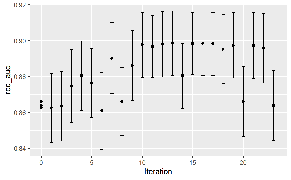
可以看出在前10次迭代就已经接近了最优指标值。
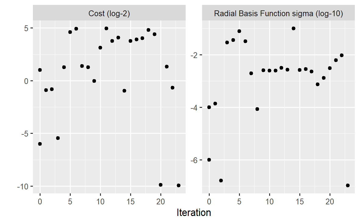
显示各次迭代的超参数点变化,这是每个超参数的变化序列:
47.5.3 模拟退火优化
模拟退火算法是一种全局优化算法, 它避免落入局部最优的做法是有一定概率跳到目标函数变差的位置。
算法基于超参数空间内的随机游动。 用随机游动在当前点局域内产生下一个候选点, 如果目标函数(性能指标)改善, 则使用下一候选点; 如果目标函数值变差, 则以一定正概率使用此候选点, 结果越差, 接受此候选点的概率也越差; 随着迭代步数的增加, 接受较差候选点的概率也随之下降。
cooling_coef控制接受较差点的概率,
此参数越小则越容易接受较差的点。
算法中如果连续出现较差的点, 则可以退回到已发现的最优点重新开始。
用finetune包的tune_sim_anneal()函数实现超参数调优的模拟退火方法。
对cells数据集,
进行参数调优:
library(finetune)
library(doParallel)

# 产生一个集群对象并注册
cl <- makePSOCKcluster(4)
registerDoParallel(cl)

ctrl_sa <- control_sim_anneal(
  verbose = TRUE,
  # 如果10步都是变差,就从已有的最优点重新开始
  no_improve = 10L)

set.seed(1404)
svm_sa <-
  svm_wflow |>
  tune_sim_anneal(
    # 指定再抽样对象,即cells的十折交叉验证数据集
    resamples = cell_folds,
    # 指定优化的性能指标,是AUC
    metrics = roc_res,
    # 用一个网格优化结果作为初值
    initial = svm_initial,
    # 指定要优化的参数、范围、变换
    param_info = svm_param,
    # 超过最大迭代步数就停止
    iter = 50,
    # 算法控制
    control = ctrl_sa
  )

# 取消集群对象
stopCluster(cl)程序中用了verbose选项详细显示迭代过程,
这些显示略去。
最后得到的AUC最优值是\(0.8985\),
与贝叶斯搜索方法AUC结果相同。
47.6 筛选许多模型
如果有多种不同的预处理方案、多个模型, 可以组成工作流程集合, 然后用再抽样技术比较这些不同的工作流程, 注意每个工作流程也需要用再抽样技术进行超参数的调优, 但从每个工作流程中选择最优的超参数组合, 也能够能对不同工作流程的性能比较。
对于不了解的数据, 一开始需要尝试很多的不同模型, 有所了解后才聚焦到少数模型, 对这些模型进行更精细的调优比较。
47.6.1 混凝土强度数据建模示例
考虑modeldata扩展包中的concrete数据。
有1030个观测,
因变量是混凝土压缩强度compressive_strength,
有7个混凝土成分变量作为自变量,
单位是每立方米千克数,
另一自变量age是测试强度等待的天数。
## Rows: 1,030
## Columns: 9
## $ cement               <dbl> 540.0, 540.0, 332.5, 332.5, 198.6, 266.0, 380.0, …
## $ blast_furnace_slag   <dbl> 0.0, 0.0, 142.5, 142.5, 132.4, 114.0, 95.0, 95.0,…
## $ fly_ash              <dbl> 0, 0, 0, 0, 0, 0, 0, 0, 0, 0, 0, 0, 0, 0, 0, 0, 0…
## $ water                <dbl> 162, 162, 228, 228, 192, 228, 228, 228, 228, 228,…
## $ superplasticizer     <dbl> 2.5, 2.5, 0.0, 0.0, 0.0, 0.0, 0.0, 0.0, 0.0, 0.0,…
## $ coarse_aggregate     <dbl> 1040.0, 1055.0, 932.0, 932.0, 978.4, 932.0, 932.0…
## $ fine_aggregate       <dbl> 676.0, 676.0, 594.0, 594.0, 825.5, 670.0, 594.0, …
## $ age                  <int> 28, 28, 270, 365, 360, 90, 365, 28, 28, 28, 90, 2…
## $ compressive_strength <dbl> 79.99, 61.89, 40.27, 41.05, 44.30, 47.03, 43.70, …
对此回归问题可以尝试许多模型, 以及许多不同的自变量选择、变换、预处理。
另外,有些观测的成分配比是相同的, 最好不要保留重复观测, 否则如果相同成分配比结果既出现在训练集又出现在测试集, 就会盲目乐观地报告模型性能, 当然, 如果在划分训练集、测试集以及划分分析集、评估集时能避免这样的问题, 也可以保留。
下面对数据进行处理, 相同配比的数据仅保留一个, 因变量值取平均值:
concrete <-
   concrete |>
   group_by(across(-compressive_strength)) |>
   summarize(
     compressive_strength = mean(compressive_strength),
     .groups = "drop")
nrow(concrete)
## [1] 992这会使得回归模型的方差齐性假设略有冲突, 但问题不大。 仅减少了38个重复观测。
按因变量分层抽样, 用\(3:1\)划分训练集、测试集, 对训练集产生重复5次的十折交叉验证集:
set.seed(1501)
concrete_split <- initial_split(
  concrete,
  strata = compressive_strength)
concrete_train <- training(concrete_split)
concrete_test  <- testing(concrete_split)

set.seed(1502)
concrete_folds <-
   vfold_cv(
     concrete_train,
     strata = compressive_strength,
     repeats = 5)
有些模型要求自变量标准化, 如神经网络、最近邻方法、支持向量机, 另外一些模型则还需要使用正交多项式变换及其交互作用效应等自变量变换。 分别产生两个食谱:
normalized_rec <-
   recipe(
     compressive_strength ~ .,
     data = concrete_train) |>
   step_normalize(all_predictors())

poly_recipe <-
   normalized_rec |>
   step_poly(all_predictors()) |>
   step_interact(~ all_predictors():all_predictors())
用parsnip扩展包为RStudio提供的addin, 可以使用鼠标菜单方法产生如下的多个模型代码, 代码略有修改:
## Warning: package 'rules' was built under R version 4.2.3##
## Attaching package: 'rules'## The following object is masked from 'package:dials':
##
## max_rules## Warning: package 'baguette' was built under R version 4.2.3# 正则化的线性回归
linear_reg_spec <-
linear_reg(
penalty = tune(),
mixture = tune()) |>
set_engine('glmnet')
# 神经网络
nnet_spec <-
mlp(
hidden_units = tune(),
penalty = tune(),
epochs = tune()) |>
set_engine('nnet') |>
set_mode('regression')
# 多元自适应回归样条
mars_spec <-
mars(
prod_degree = tune()) |>
set_engine('earth') |>
set_mode('regression')
# 支持向量机,使用径向基
svm_r_spec <-
svm_rbf(
cost = tune(),
rbf_sigma = tune() ) |>
set_engine('kernlab') |>
set_mode('regression')
# 支持向量机,使用多项式基
svm_p_spec <-
svm_poly(
cost = tune(),
degree = tune() ) |>
set_engine('kernlab') |>
set_mode('regression')
# 最近邻方法
knn_spec <-
nearest_neighbor(
neighbors = tune(),
weight_func = tune(),
dist_power = tune()) |>
set_engine('kknn') |>
set_mode('regression')
# 回归判别树
cart_spec <-
decision_tree(
min_n = tune(),
cost_complexity = tune()) |>
set_engine('rpart') |>
set_mode('regression')
# 装袋法
bag_cart_spec <-
bag_tree() |>
set_engine('rpart', times = 50L) |>
set_mode('regression')
# 随机森林
rf_spec <-
rand_forest(
mtry = tune(),
min_n = tune(),
trees = 1000) |>
set_engine('ranger') |>
set_mode('regression')
# XGBOOST
xgb_spec <-
boost_tree(
tree_depth = tune(),
trees = tune(),
learn_rate = tune(),
min_n = tune(),
loss_reduction = tune(),
sample_size = tune()) |>
set_engine('xgboost') |>
set_mode('regression')
# 基于规则的模型
cubist_spec <-
cubist_rules(
committees = tune(),
neighbors = tune()) |>
set_engine('Cubist')对神经网络方法, 根据已有分析, 设置隐藏单元个数至多27个:
47.6.2 生成工作流程集合
上面提供了许多种模型, 不同的模型需要不同的预处理, 用工作流程集合将预处理和模型匹配。
先生成仅需要标准化自变量的工作流程集合:
normalized <-
   workflow_set(
      preproc = list(
        normalized = normalized_rec),
      models = list(
        SVM_radial = svm_r_spec,
        SVM_poly = svm_p_spec,
        KNN = knn_spec,
        neural_network = nnet_spec) )
normalized
## # A workflow set/tibble: 4 × 4
## wflow_id info option result
## <chr> <list> <list> <list>
## 1 normalized_SVM_radial <tibble [1 × 4]> <opts[0]> <list [0]>
## 2 normalized_SVM_poly <tibble [1 × 4]> <opts[0]> <list [0]>
## 3 normalized_KNN <tibble [1 × 4]> <opts[0]> <list [0]>
## 4 normalized_neural_network <tibble [1 × 4]> <opts[0]> <list [0]>上面仅指定了一种预处理, 所以指定的4个模型都使用这种预处理。 如果指定了多种预处理, 默认会与模型进行两两交叉。
结果中wflow_id列用来区分不同的工作流程,
可以用extract_workflow()指定某一工作流程提取出来:
## ══ Workflow ════════════════════════════════════════════════════════════════════
## Preprocessor: Recipe
## Model: nearest_neighbor()
##
## ── Preprocessor ────────────────────────────────────────────────────────────────
## 1 Recipe Step
##
## • step_normalize()
##
## ── Model ───────────────────────────────────────────────────────────────────────
## K-Nearest Neighbor Model Specification (regression)
##
## Main Arguments:
##   neighbors = tune()
##   weight_func = tune()
##   dist_power = tune()
##
## Computational engine: kknn工作流程集合的info列是保存具体工作流程信息的tibble数据框,
option列保存工作流程调优时需要的参数,
如预处理用的超参数和模型估计用的超参数,
当前是空置的,
可以用options_add()增加这样的选项,
如:
normalized <-
   normalized |>
   option_add(
     param_info = nnet_param,
     id = "normalized_neural_network")
normalized
## # A workflow set/tibble: 4 × 4
## wflow_id info option result
## <chr> <list> <list> <list>
## 1 normalized_SVM_radial <tibble [1 × 4]> <opts[0]> <list [0]>
## 2 normalized_SVM_poly <tibble [1 × 4]> <opts[0]> <list [0]>
## 3 normalized_KNN <tibble [1 × 4]> <opts[0]> <list [0]>
## 4 normalized_neural_network <tibble [1 × 4]> <opts[1]> <list [0]>工作流程集合中的result列用来保存拟合或者评估结果,
目前为空置。
工作流程集合除了使用食谱指定变量和变量变换, 还可以使用dplyr方式指定变量。 比如, 下面的程序仅指定因变量、自变量, 以及不需要特殊处理的一些模型, 组成工作流程集合:
model_vars <-
   workflow_variables(
     outcomes = compressive_strength,
     predictors = everything())

no_pre_proc <-
   workflow_set(
      preproc = list(simple = model_vars),
      models = list(
        MARS = mars_spec,
        CART = cart_spec,
        CART_bagged = bag_cart_spec,
        RF = rf_spec,
        boosting = xgb_spec,
        Cubist = cubist_spec) )
no_pre_proc
## # A workflow set/tibble: 6 × 4
## wflow_id info option result
## <chr> <list> <list> <list>
## 1 simple_MARS <tibble [1 × 4]> <opts[0]> <list [0]>
## 2 simple_CART <tibble [1 × 4]> <opts[0]> <list [0]>
## 3 simple_CART_bagged <tibble [1 × 4]> <opts[0]> <list [0]>
## 4 simple_RF <tibble [1 × 4]> <opts[0]> <list [0]>
## 5 simple_boosting <tibble [1 × 4]> <opts[0]> <list [0]>
## 6 simple_Cubist <tibble [1 × 4]> <opts[0]> <list [0]>下面生成需要标准化和正交多项式扩展、交互作用的模型集合:
with_features <-
   workflow_set(
      preproc = list(
        full_quad = poly_recipe),
      models = list(
        linear_reg = linear_reg_spec,
        KNN = knn_spec) )
上面生成了三个工作流程集合, 将其合并成一个大的工作流程集合:
all_workflows <-
   bind_rows(
     no_pre_proc,
     normalized,
     with_features) |>
   # 简化工作流程的id:
   mutate(
     wflow_id = gsub(
       "(simple_)|(normalized_)", "", wflow_id))
all_workflows
## # A workflow set/tibble: 12 × 4
## wflow_id info option result
## <chr> <list> <list> <list>
## 1 MARS <tibble [1 × 4]> <opts[0]> <list [0]>
## 2 CART <tibble [1 × 4]> <opts[0]> <list [0]>
## 3 CART_bagged <tibble [1 × 4]> <opts[0]> <list [0]>
## 4 RF <tibble [1 × 4]> <opts[0]> <list [0]>
## 5 boosting <tibble [1 × 4]> <opts[0]> <list [0]>
## 6 Cubist <tibble [1 × 4]> <opts[0]> <list [0]>
## 7 SVM_radial <tibble [1 × 4]> <opts[0]> <list [0]>
## 8 SVM_poly <tibble [1 × 4]> <opts[0]> <list [0]>
## 9 KNN <tibble [1 × 4]> <opts[0]> <list [0]>
## 10 neural_network <tibble [1 × 4]> <opts[1]> <list [0]>
## 11 full_quad_linear_reg <tibble [1 × 4]> <opts[0]> <list [0]>
## 12 full_quad_KNN <tibble [1 × 4]> <opts[0]> <list [0]>47.6.3 模型调优与比较
工作流程集合中的大多数工作流程都含有需要调节的超参数,
可以用workflow_map()就某个调优函数应用到每个工作流程,
默认使用tune_grid()函数。
本例使用非规则网格调优方法, 每个工作流程最多使用25个网格点。 因为都是回归类型的模型, 所以可以有一些共同的输入, 比如再抽样集合、性能指标。
library(doParallel)

# 网格搜索共用的选项
grid_ctrl <- control_grid(
      save_pred = TRUE,
      parallel_over = "everything",
      save_workflow = TRUE )

# 产生一个集群对象并注册
cl <- makePSOCKcluster(6)
registerDoParallel(cl)

time0 <- proc.time()[3]
# 实际对每个工作流程进行调优
grid_results <-
  all_workflows |>
  workflow_map(
    seed = 1503,
    resamples = concrete_folds,
    grid = 25,
    control = grid_ctrl  )
time1 <- proc.time()[3] - tim0
cat("用时:", time1, "秒\n")

# 取消集群对象
stopCluster(cl)
上面的多个模型的超参数调优计算量很大, 共有12600次模型拟合与预报, 需要运行几个小时的时间。
要注意的是, 这不仅对每个工作流程进行了超参数调优, 而且只要对每个工作流程选择最优的超参数方案, 就可以比较不同工作流程的性能。 当然, 因为模型太多, 所以网格法参数调优不能使用太多的计算量, 超参数调优不能进行得很精细, 可以排除表现很差的模型, 性能排在前列的模型的比较次序并不能完全确定。
rank_results()可以提取某个性能指标进行模型间的比较,
回归问题的默认性能指标是RMSE,
显示表现较好的若干模型:
grid_results |>
   rank_results(select_best=TRUE) |>
   filter(.metric == "rmse") |>
   select(model, .config, rmse = mean, rank)
结果略。
作图显示模型比较:
autoplot(
   grid_results,
   rank_metric = "rmse",  # 模型间比较的性能指标
   metric = "rmse",       # 用来可视化的性能指标
   select_best = TRUE     # 对每个工作流程仅显示最优超参数组合
   ) +
   geom_text(
   aes(y = mean - 1/2, label = wflow_id),
   angle = 90, hjust = 1) +
   lims(y = c(3.5, 9.5)) +
   theme(legend.position = "none")
图形略。 最优模型是XGBOOST。
对某个工作流程作超参数调优的图形:
autoplot(grid_results,
  id = "Cubist", metric = "rmse")
对工作流程集合的调优结果,
仍可以使用collect_predictions()函数提取每个工作流程在每个折上的预测值,
使用collect_metrics()提取每个工作流程在每个折上的性能指标。
47.6.4 加速模型调优
对一大批模型进行超参数调优要耗费很长时间, 而且每个模型的调优都不能进行得很精细。 可以用赛跑方法在调优过程中放弃表现很差的模型。
workflow_map()默认使用非规则网格点方法进行每个模型的超参数调优,
但是也可以使用tune_race_anova(),
这时在对每个模型调优时,
可以提前放弃表现很差的超参数组合。
library(doParallel)
library(finetune)

# 网格赛跑调优共用的选项
race_ctrl <- control_race(
  save_pred = TRUE,
  parallel_over = "everything",
  save_workflow = TRUE )

# 产生一个集群对象并注册
cl <- makePSOCKcluster(6)
registerDoParallel(cl)

time0 <- proc.time()[3]
# 实际对每个工作流程进行调优
race_results <-
  all_workflows |>
  workflow_map(
    "tune_race_anova",
    seed = 1503,
    resamples = concrete_folds,
    grid = 25,
    control = race_ctrl )
time1 <- proc.time()[3] - time0
cat("用时:", time1, "秒\n")

# 取消集群对象
stopCluster(cl)
上述程序进行了1050个模型拟合, 计算量降低了一个数量级。 仅用时10分钟。
结果是一个数据框格式,
每个工作流程占一行,
其中的results列会显示race[+],
这是使用了赛跑算法的结果:
# A workflow set/tibble: 12 × 4
   wflow_id             info             option    result
   <chr>                <list>           <list>    <list>
 1 MARS                 <tibble [1 × 4]> <opts[3]> <race[+]>
 2 CART                 <tibble [1 × 4]> <opts[3]> <race[+]>
 3 CART_bagged          <tibble [1 × 4]> <opts[3]> <rsmp[+]>
 4 RF                   <tibble [1 × 4]> <opts[3]> <race[+]>
 5 boosting             <tibble [1 × 4]> <opts[3]> <race[+]>
 6 Cubist               <tibble [1 × 4]> <opts[3]> <race[+]>
 7 SVM_radial           <tibble [1 × 4]> <opts[3]> <race[+]>
 8 SVM_poly             <tibble [1 × 4]> <opts[3]> <race[+]>
 9 KNN                  <tibble [1 × 4]> <opts[3]> <race[+]>
10 neural_network       <tibble [1 × 4]> <opts[4]> <race[+]>
11 full_quad_linear_reg <tibble [1 × 4]> <opts[3]> <race[+]>
12 full_quad_KNN        <tibble [1 × 4]> <opts[3]> <race[+]>
注意上述结果没有按性能指标排序。
作图比较各个模型:
autoplot(
  race_results,
  rank_metric = "rmse",
  metric = "rmse",
  select_best = TRUE) +
  geom_text(aes(
    y = mean - 1/2, label = wflow_id),
    angle = 90, hjust = 1) +
  lims(y = c(3.0, 9.5)) +
  theme(legend.position = "none")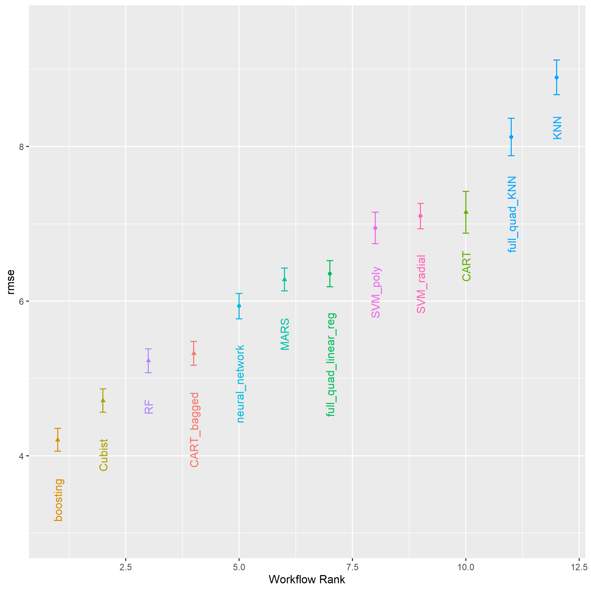
图形略。 仍是XGBOOST最优, Cubist次之。
将赛跑方法与仅使用网格搜索的方法结果比较, 可以发现各个工作流程选用的最优超参数组合一致的比例不到一半, 但是两种方法估计的性能指标基本相等, 两种方法的性能指标的相关系数达到\(0.968\)。 实际上, 不同的超参数组合都有可能达到相近的预测性能。
47.6.5 选定最终的模型
在对所有模型调优后, 应该选定一个最优的模型(工作流程), 在训练集上进行拟合, 在测试集上进行性能评估。 这与对单个模型的做法类似。
因为比较结果是XGBOOST模型最优, 所以提取此模型的超参数设置:
best_results <-
  race_results |>
  # 提取一个工作流程的调优结果
  extract_workflow_set_result("boosting") |>
  # 从调优结果中选择最优的超参数组合
  select_best(metric = "rmse")
best_results
# A tibble: 1 × 7
trees min_n tree_depth learn_rate loss_reduction
<int> <int> <int> <dbl> <dbl>
1 1957 8 7 0.0756 0.000000145
# ℹ 2 more variables: sample_size <dbl>, .config <chr>用最优模型在整个训练集上拟合, 在测试集上预测:
boosting_test_results <-
  race_results |>
  extract_workflow("boosting") |>
  finalize_workflow(best_results) |>
last_fit(split = concrete_split)用collect_metrics()提取测试集上的性能指标:
# A tibble: 2 × 4
  .metric .estimator .estimate .config
  <chr>   <chr>          <dbl> <chr>
1 rmse    standard       3.41  Preprocessor1_Model1
2 rsq standard 0.954 Preprocessor1_Model1用collect_predictions()提取测试集上的预测值,
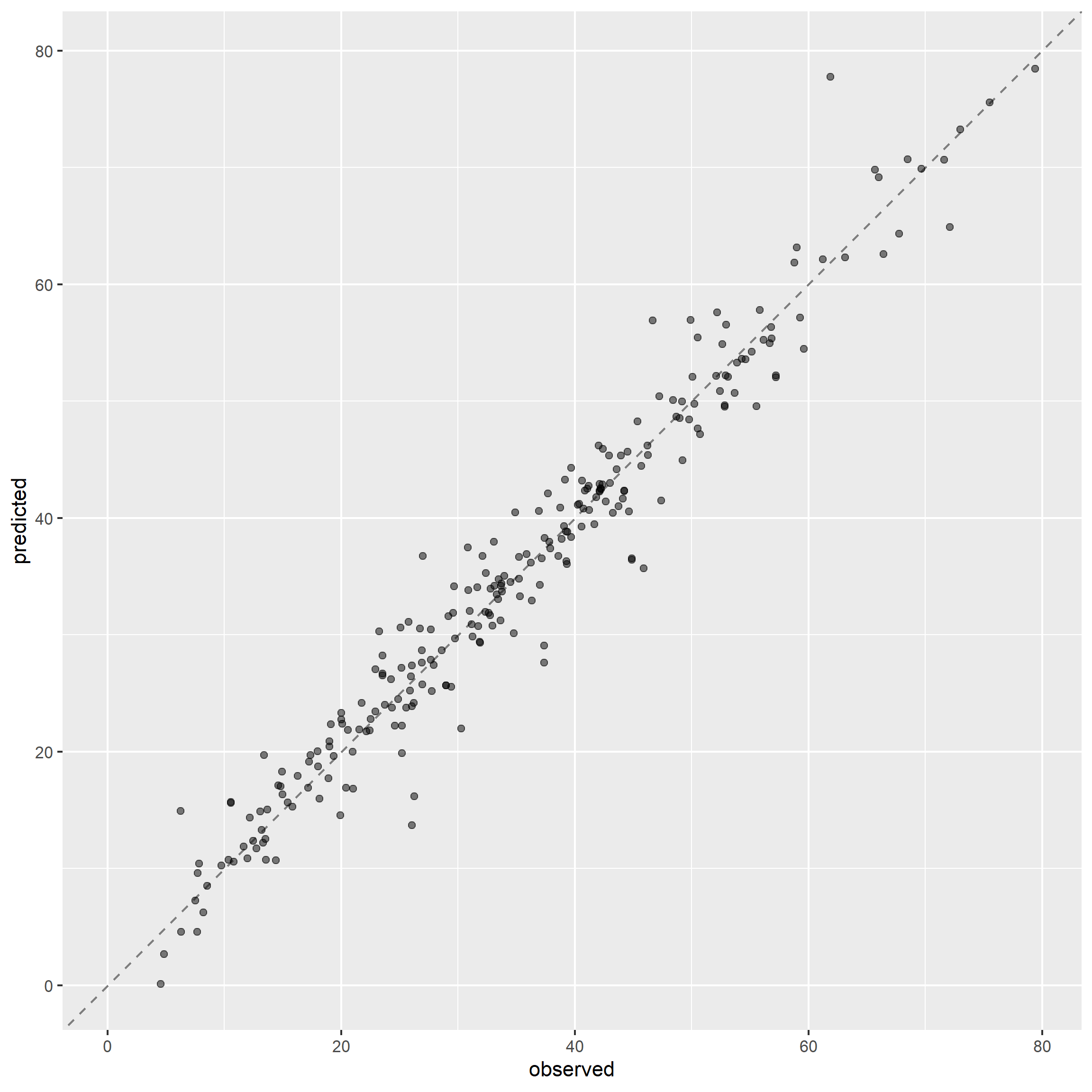
与真实值对比作图:
boosting_test_results |>
  collect_predictions() |>
  ggplot(aes(
    x = compressive_strength, y = .pred)) +
  # 作y=x直线
  geom_abline(color = "gray50", lty = 2) +
  geom_point(alpha = 0.5) +
  coord_obs_pred() +
  labs(x = "observed", y = "predicted")