31 使用infer包进行统计推断
R的infer扩展包提供了与tidyverse系统习惯做法一致的进行假设检验的方法。 在进行理论推断时, 主要使用随机模拟方法进行计算, 也支持基于理论分布的方法。 这个包的当前版本(1.2.9001)还有一些错误, 不能用于较正式的研究问题。
以数据框(tibble)为输入,
用动词specify指定针对的变量,
用hypothesis指定假设检验(包括置信区间所针对的参数),
用generate生成零假设下的多组模拟样本(可以是bootstrap样本,
也可以是理论分布而不需要模拟),
用calculate计算统计量或者对多组模拟样本计算产生满足检验统计量(或枢轴量)抽样分布的随机样本,
或者用assume指定理论抽样分布。
从抽样分布的样本或理论分布,
可以用visualize查看抽样分布直方图,
用shaded_p_value在抽样分布直方图中标出统计量值位置并加亮显示p值对应面积,
用get_p_value计算p值,
用get_confidence_interval计算置信区间,
用shaded_confidence_interval在抽样分布直方图中加亮显示置信区间。
31.1 单样本均值的比较
考虑咖啡标重的检验问题。
31.1.1 随机模拟方法
infer包主要使用随机模拟方法生成多组随机样本, 产生服从检验统计量抽样分布的样本, 然后计算推断结果。
计算样本均值:
## Response: Weight (numeric)
## # A tibble: 1 × 1
##    stat
##   <dbl>
## 1 2.92用specify在数据框中指定要分析的变量。
在calculate中指定为stat = "mean",
则计算均值统计量。
用bootstrap方法生成多组样本, 然后对每个样本计算样本均值, 得到服从检验统计量抽样分布的样本(近似):
null_dist <- Coffee |>
  specify(response = Weight) |>
  hypothesize(null = "point", mu = 3) |>
  generate(reps = 1000) |>
  calculate(stat = "mean")
## Setting `type = "bootstrap"` in `generate()`.hypothesize()中的null = "point",
就是指单样本的某个参数的检验问题,
用mu = 3指定了零假设是\(H_0: \mu = 3\)。
用generate()按照bootstrap方法生成多组再抽样随机样本。
用calculate()对每一组再抽样随机样本计算均值统计量,
作为bootstrap方法得到的样本均值的抽样分布近似。
计算左侧p值:
## # A tibble: 1 × 1
##   p_value
##     <dbl>
## 1   0.002
程序中输入了均值统计量的bootstrap分布(用一个很大的bootstrap均值统计量的随机样本代表)和实际数据的均值统计量,
计算了实际数据的均值统计量在bootstrap分布中的左侧概率作为p值。
direction可取"less"(左侧)、"greater"(右侧)和"two-sided"(双侧,或"both")。
对\(\bar x\)抽样分布(bootstrap近似)抽样分布作直方图, 并标出\(\bar x\)值, 高亮显示p值对应的面积:

计算置信区间, 用bootstrap样本分位数:
## # A tibble: 1 × 2
##   lower_ci upper_ci
##      <dbl>    <dbl>
## 1     2.95     3.06
计算置信区间, 用bootstrap样本计算的标准误差:
## # A tibble: 1 × 2
##   lower_ci upper_ci
##      <dbl>    <dbl>
## 1     2.87     2.97
置信区间作图:
ci <- null_dist |>
  get_confidence_interval(
    level = 0.95, type = "percentile")
null_dist |>
  visualise() +
  shade_confidence_interval(ci)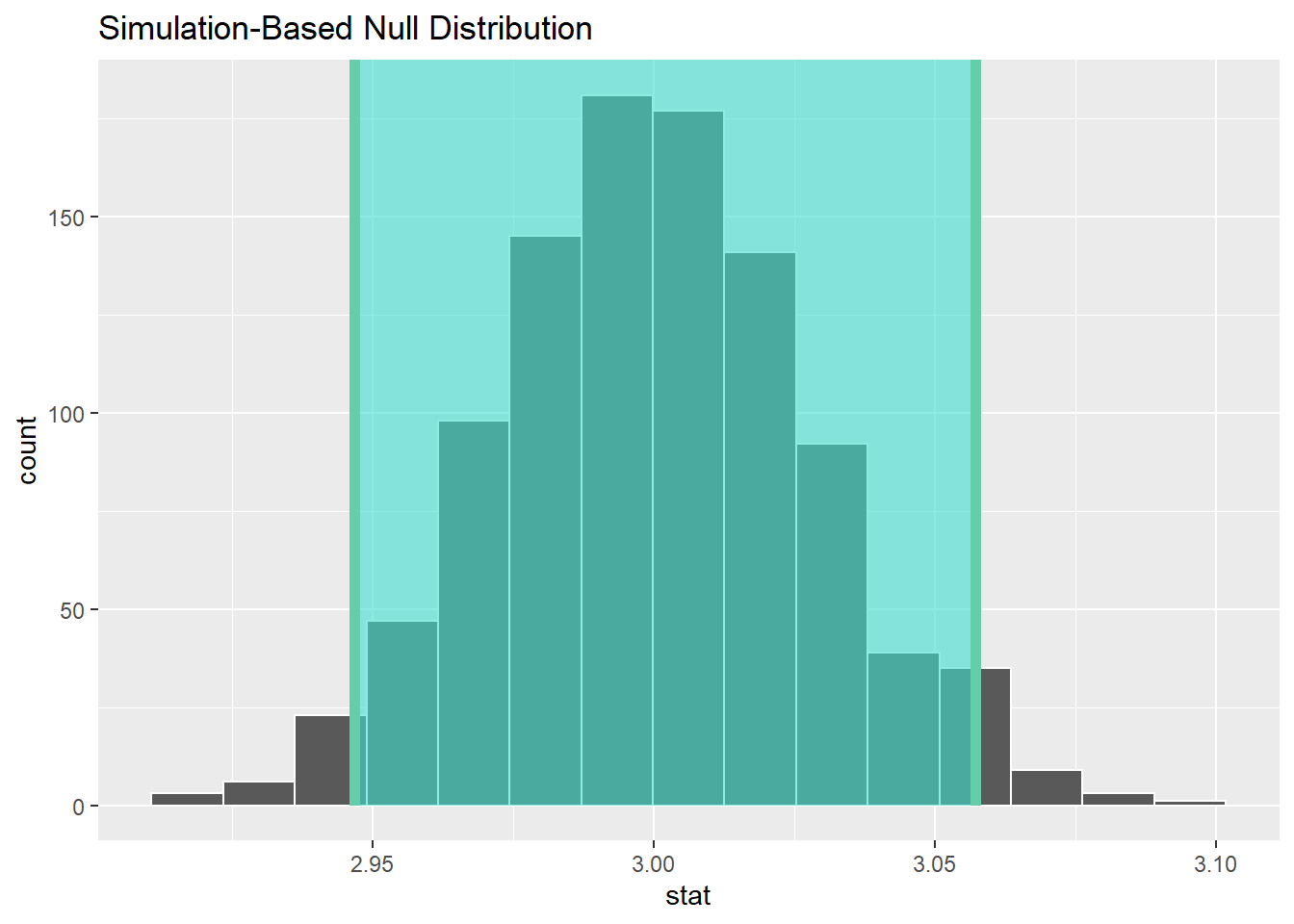
31.1.2 理论方法
用t检验的理论方法, 先计算统计量:
t_stat <- Coffee |>
  specify(response = Weight) |>
  hypothesize(null = "point", mu = 3) |>
  calculate(stat = "t")
t_stat
## Response: Weight (numeric)
## Null Hypothesis: point
## # A tibble: 1 × 1
## stat
## <dbl>
## 1 -2.82指定检验统计量理论分布:
计算左侧检验的p值:
## # A tibble: 1 × 1
##   p_value
##     <dbl>
## 1 0.00389
p值为0.004, 在0.01水平下拒绝零假设, 认为该品牌咖啡实际重量显著低于标称重量。
计算\(\mu\)的置信区间:
xbar <- Coffee |>
  specify(response = Weight) |>
  calculate(stat = "mean")
t_dist |>
  get_confidence_interval(level = 0.95,
    point_estimate = xbar)
## # A tibble: 1 × 2
## lower_ci upper_ci
## <dbl> <dbl>
## 1 2.86 2.98作统计量抽样分布图, 并标出统计量值, 加亮显示p值对应面积:
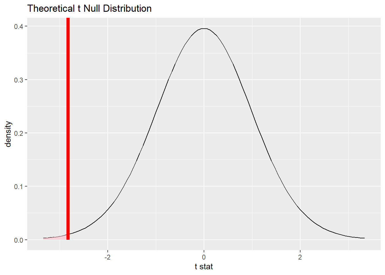
注意visualize和shade_p_value之间用+号而不是|>连接。
作置信区间图并与\(\bar x\)抽样分布叠加:
xbar <- Coffee |>
  specify(response = Weight) |>
  calculate(stat = "mean")
ci <- t_dist |>
  get_confidence_interval(level = 0.95,
    point_estimate = xbar)
t_dist |>
  visualise() +
  shade_confidence_interval(ci)
函数t_test()提供了t检验和置信区间计算功能,如:
## # A tibble: 1 × 7
##   statistic  t_df p_value alternative estimate lower_ci upper_ci
##       <dbl> <dbl>   <dbl> <chr>          <dbl>    <dbl>    <dbl>
## 1     -2.82    35 0.00389 less            2.92     -Inf     2.97
31.2 独立两样本均值比较
考虑前面的两个银行营业所账户平均存款比较问题。 需要将数据转换为长表格式, 即分组变量占一列, 存款占一列:
da_bank <- CheckAcct |>
  pivot_longer(all_of(c("Cherry Grove", "Beechmont")),
    names_to = "Shop",
    values_to = "Balance",
    values_drop_na = TRUE)
计算均值的差:
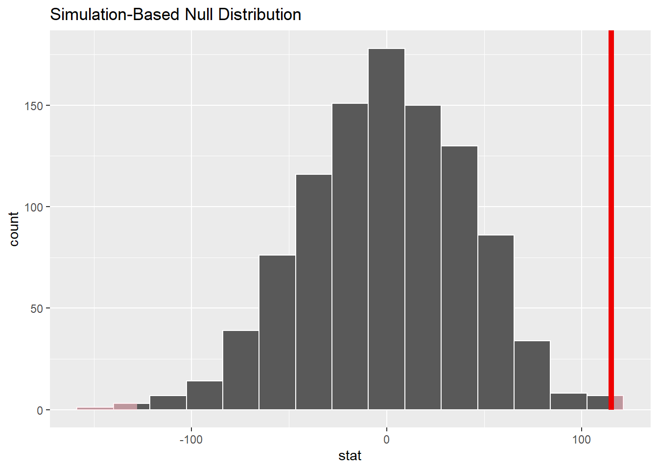
obs_stat <- da_bank |>
  specify(Balance ~ Shop) |>
  calculate(stat = "diff in means",
    order = c("Cherry Grove", "Beechmont"))
obs_stat
## Response: Balance (numeric)
## Explanatory: Shop (factor)
## # A tibble: 1 × 1
## stat
## <dbl>
## 1 115.在calculate中指定了要计算的统计量是均值的差,
并且次序是"Cherry Grove"营业所均值减去"Beechmont"营业所均值。
用两组随机置换方法生成多组随机样本, 作为零假设下的样本, 计算多个均值差统计量, 代表零假设下均值差统计量的分布:
null_dist <- da_bank |>
  specify(Balance ~ Shop) |>
  hypothesize(null = "independence") |>
  generate(reps = 1000) |>
  calculate(stat = "diff in means",
    order = c("Cherry Grove", "Beechmont"))
## Setting `type = "permute"` in `generate()`.其中hypothesize(null = "independence")表示零假设是独立两组比较问题,
这里配合calculate中stat = "diff in means",
可知零假设是独立两组均值的比较问题。
generate()生成零假设下的多个样本,
使用了置换检验方法,
即保持样本中Balance(账户存款额)不变,
但是将所有\(n\)个(\(n\)为样本量)营业所标签(Shop)随机打乱重排,
这样就抹去了两个营业所的区别,
得到的新样本代表了零假设成立情况下的分布。
计算双侧检验p值:
## # A tibble: 1 × 1
##   p_value
##     <dbl>
## 1   0.006
这是独立两组均值比较的置换检验方法。 置换检验不需要通常的基于理论的独立两样本t检验方法要求两组服从正态分布以及方差相等等前提, 仍需要假定两组独立。 所以置换检验比独立两样本t检验更为适用。
作两均值统计量差的零假设下分布直方图, 并标出p值对应的面积:
infer也提供了作独立两样本t检验的函数t_test(),如:
## # A tibble: 1 × 7
##   statistic  t_df p_value alternative estimate lower_ci upper_ci
##       <dbl> <dbl>   <dbl> <chr>          <dbl>    <dbl>    <dbl>
## 1      2.96  47.8 0.00483 two.sided       115.     36.8     193.
31.3 成对均值比较
成对均值比较, 实际是成对均值的差值与0的比较。
以前面两种工艺时间的比较为例。 使用单样本的bootstrap检验。
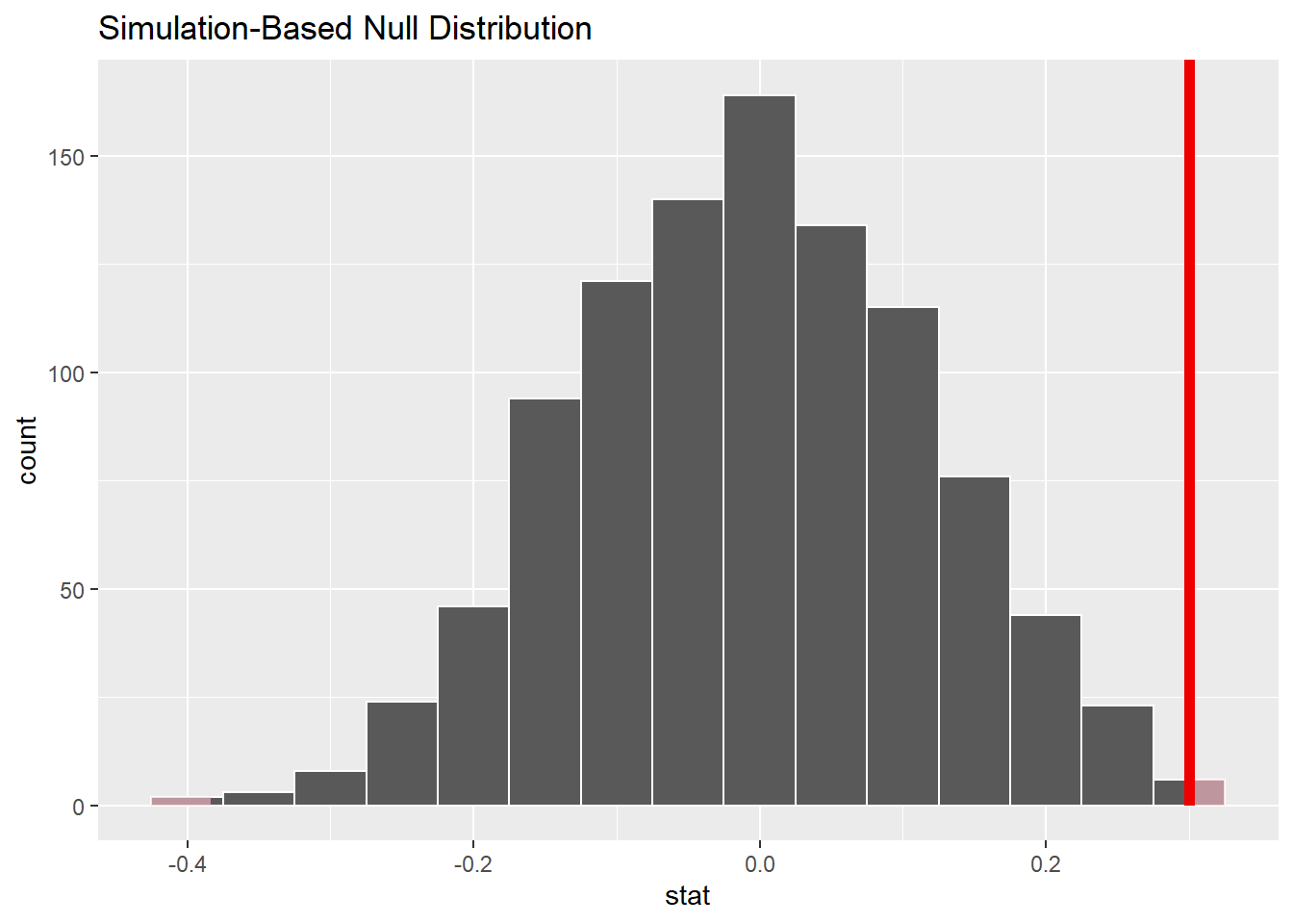
计算成对的差值, 以及差值的均值:
da_proc <- Matched |>
  mutate(time_diff = `Method 1` -`Method 2`)
diff_mean <- da_proc |>
  specify(response = time_diff) |>
  calculate(stat = "mean")
diff_mean
## Response: time_diff (numeric)
## # A tibble: 1 × 1
## stat
## <dbl>
## 1 0.3生成bootstrap样本:
boot_dist <- da_proc |>
  specify(response = time_diff) |>
  hypothesize(null = "point", mu = 0) |>
  generate(reps = 1000) |>
  calculate(stat = "mean")
## Setting `type = "bootstrap"` in `generate()`.计算双侧p值:
## # A tibble: 1 × 1
##   p_value
##     <dbl>
## 1   0.002
图示:
31.4 单样本比例的比较
为了使用随机模拟方法, 需要有二值(是、否)的观测样本。 可以从汇总统计反向生成这样的样本。
考虑前面的高尔夫培训女生比例的例子。 按汇总数据生成原始数据:
计算比例统计量:
## Response: gender (factor)
## # A tibble: 1 × 1
##    stat
##   <dbl>
## 1  0.25
生成满足零假设的多组样本(真实比例为0.20的样本), 从每个样本计算比例统计量并作图:
null_dist <- FemGolf |>
  specify(response = gender, success = "F") |>
  hypothesize(null = "point", p = 0.20) |>
  generate(reps = 1000) |>
  calculate(stat = "prop")
## Setting `type = "draw"` in `generate()`.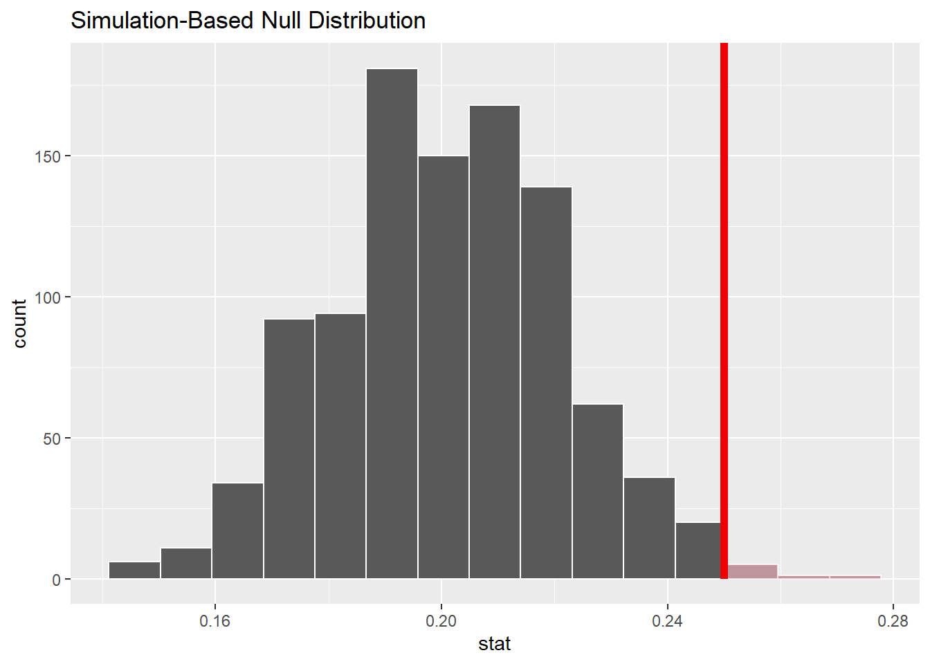
显示p值:
## # A tibble: 1 × 1
##   p_value
##     <dbl>
## 1   0.007
在0.05水平下拒绝零假设, 认为女性学员比例显著增加了。
用bootstrap和bootstrap样本的分位数计算双侧置信区间:
FemGolf |>
  specify(response = gender, success = "F") |>
  generate(reps = 1000, type="bootstrap") |>
  calculate(stat = "prop") |>
  get_confidence_interval(level = 0.95,
    type = "percentile")
## # A tibble: 1 × 2
## lower_ci upper_ci
## <dbl> <dbl>
## 1 0.208 0.292用零假设下样本和标准误差计算双侧置信区间:
FemGolf |>
  specify(response = gender, success = "F") |>
  hypothesize(null = "point", p = 0.20) |>
  generate(reps = 1000, type="draw") |>
  calculate(stat = "prop") |>
  get_confidence_interval(level = 0.95,
    type = "se",
    point_estimate = p_stat)
## # A tibble: 1 × 2
## lower_ci upper_ci
## <dbl> <dbl>
## 1 0.209 0.29131.5 独立两样本比例的比较
如果只有汇总数据, 为了使用随机模拟方法(再抽样方法), 还需要制作原始观测数据集。
考虑前面的报税代理分理处的错误率比较问题。 制作样本数据集:
da_tax <- tibble(
  shop = factor(rep(c(1,2), c(250, 300))),
  error = factor(rep(c("yes", "no", "yes", "no"),
    c(35, 250-35, 27, 300-27)),
    levels = c("yes", "no")) )
计算错误率差的统计量:
obs_stat <- da_tax |>
  specify(error ~ shop, success = "yes") |>
  calculate(stat = "diff in props",
    order = c(1, 2))
obs_stat
## Response: error (factor)
## Explanatory: shop (factor)
## # A tibble: 1 × 1
## stat
## <dbl>
## 1 0.05上面的specify用了y ~ g的格式给出了分组变量g和二值变量y,
并用success指定了二值变量y作为两点分布观测值时,
哪一个值当作成功。
用随机重排方法产生多个模拟样本, 对每个样本计算比例差统计量, 作为零假设下的统计量样本。 所谓随机重排, 是指保持样本量不变, 两个分理处的观测数\(n_1\)和\(n_2\)不变, 但将所有\(n=n_1 + n_2\)个观测随机地重新标\(n_1\)个为分理处1, \(n_2\)个为分理处2。 这样的样本就代表两个分理处是不区分的, 即代表了零假设成立情况下的样本。
null_dist <- da_tax |>
  specify(error ~ shop, success = "yes") |>
  hypothesize(null = "independence") |>
  generate(reps = 1000) |>
  calculate(stat = "diff in props",
    order = c(1, 2))
## Setting `type = "permute"` in `generate()`.上面的程序的hypothesize中null = "independence"表示要检验的零假设是两组比较问题,
对比例比较问题,
零假设就是独立两组的比例相等。
双侧检验:
## # A tibble: 1 × 1
##   p_value
##     <dbl>
## 1    0.08
这种检验方法称为“置换检验”(permutation test)。
利用比例差的统计量值, 以及从零假设下置换检验方法生成的统计量分布计算到标准误差, 计算比例差的置信区间:
## # A tibble: 1 × 2
##   lower_ci upper_ci
##      <dbl>    <dbl>
## 1 -0.00229    0.102
为了计算置信区间, 也可以使用bootstrap方法产生样本, 用bootstrap样本的统计量抽样分布的分位数计算置信区间:
da_tax |>
  specify(error ~ shop, success = "yes") |>
  generate(reps = 1000, type = "bootstrap") |>
  calculate(stat = "diff in props",
    order = c(1, 2)) |>
  get_confidence_interval(
    level = 0.95,
    type = "percentile")
## # A tibble: 1 × 2
## lower_ci upper_ci
## <dbl> <dbl>
## 1 -0.00368 0.105或利用比例差统计量和从bootstrap样本中估计的标准误差计算置信区间:
da_tax |>
  specify(error ~ shop, success = "yes") |>
  generate(reps = 1000, type = "bootstrap") |>
  calculate(stat = "diff in props",
    order = c(1, 2)) |>
  get_confidence_interval(
    level = 0.95,
    type = "se",
    point_estimate = obs_stat)
## # A tibble: 1 × 2
## lower_ci upper_ci
## <dbl> <dbl>
## 1 -0.00225 0.10231.6 拟合优度检验
!!!当前infer扩展包(1.2.1.9001)的拟合优度代码可能有误,卡方统计量计算错误!!
考虑前面的5个候选人, 甲和乙支持率相等的零假设。 通过汇总数据生成原始数据集:
计算拟合优度卡方统计量:
chisq_stat <- da_poll |>
  specify(response = support) |>
  hypothesize(null = "point", p = c(
    "A" = 0.25,
    "B" = 0.25,
    "Other" = 0.5  )) |>
  calculate(stat = "Chisq")
chisq_stat
## Response: support (factor)
## Null Hypothesis: point
## # A tibble: 1 × 1
## stat
## <dbl>
## 1 20生成零假设下的样本:
null_dist <- da_poll |>
  specify(response = support) |>
  hypothesize(null = "point", p = c(
    "A" = 0.25,
    "B" = 0.25,
    "Other" = 0.5  )) |>
  generate(reps = 1000, type = "draw") |>
  calculate(stat = "Chisq")
null_dist |>
  visualize() +
  shade_p_value(
    obs_stat = chisq_stat,
    direction = "greater"  )
计算p值:
## Warning: Please be cautious in reporting a p-value of 0. This result is an
## approximation based on the number of `reps` chosen in the `generate()` step.
## See `?get_p_value()` for more information.
## # A tibble: 1 × 1
## p_value
## <dbl>
## 1 031.7 列联表独立性检验
独立两样本比例比较可以看成是列联表独立性检验的特例。 考虑前面的不同性别对啤酒种类偏好差异的例子。 为了使用随机模拟方法, 从表格数据生成具体的观测数据集:
ctab.beer <- rbind(c(
20, 40, 20),
c(30,30,10))
colnames(ctab.beer) <- c("Light", "Regular", "Dark")
rownames(ctab.beer) <- c("Male", "Female")
d1 <- expand_grid(
gender = factor(
c("Male", "Female"), levels=c("Male", "Female")),
beer = factor(
c("Light", "Regular", "Dark"),
levels=c("Light", "Regular", "Dark"))) |>
mutate(n = c(t(ctab.beer)))
da_beer <- tibble(
gender = rep(d1$gender, d1$n),
beer = rep(d1$beer, d1$n))
da_beer |> count(gender, beer)## # A tibble: 6 × 3
## gender beer n
## <fct> <fct> <int>
## 1 Male Light 20
## 2 Male Regular 40
## 3 Male Dark 20
## 4 Female Light 30
## 5 Female Regular 30
## 6 Female Dark 10计算卡方统计量:
## Response: beer (factor)
## Explanatory: gender (factor)
## # A tibble: 1 × 1
## stat
## <dbl>
## 1 6.12用置换检验, 将数据中的性别随机重排, 生成多组重抽样样本, 对每个样本计算卡方统计量, 作为独立零假设下统计量分布的近似:
null_dist <- da_beer |>
specify(beer ~ gender) |>
hypothesize(null = "independence") |>
generate(reps = 1000) |>
calculate(stat = "Chisq")## Setting `type = "permute"` in `generate()`.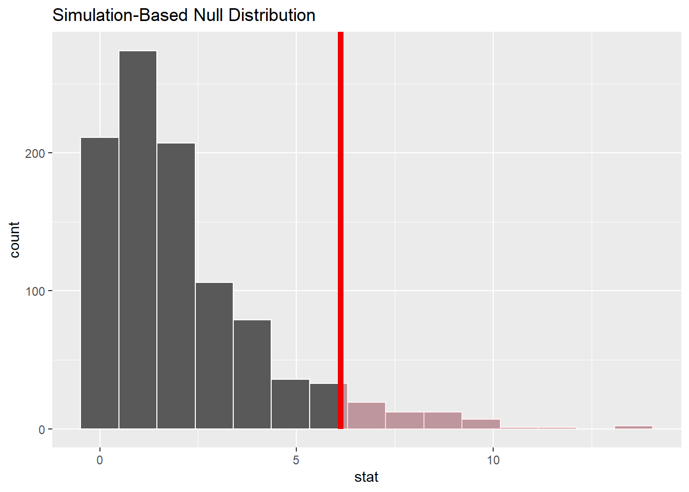
计算p值:
## # A tibble: 1 × 1
##   p_value
##     <dbl>
## 1 0.059也可以使用理论卡方分布检验:
null_dist_th <- da_beer |>
  specify(beer ~ gender) |>
  assume(distribution = "Chisq")
null_dist_th |>
  visualize() +
  shade_p_value(
    obs_stat = chisq_stat,
    direction = "greater"
  )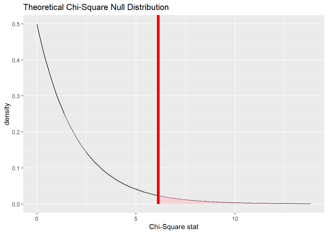
## # A tibble: 1 × 1
##   p_value
##     <dbl>
## 1  0.0468
或:
## # A tibble: 1 × 3
##   statistic chisq_df p_value
##       <dbl>    <int>   <dbl>
## 1      6.12        2  0.0468