23 其它的波动率计算方法
本章内容来自自(Tsay 2013)§4.15和§4.16内容。
23.1 利用日频计算月频波动率
(French, Schwert, and Stambaugh 1987)用高频数据计算低频收益率的波动率, 又可参见(Andersen et al. 2001)和(Andersen et al. 2001)。
假设我们对某资产的月波动率感兴趣, 有该资产的日收益率数据, 设\(r_t^m\)是该资产第\(t\)个月的对数收益率, 第\(t\)个月共有\(n\)个交易日, 所有日对数收益率为\(\{ r_{t,i} \}_{i=1}^n\), 则 \[ r_t^m = \sum_{i=1}^n r_{t,i} . \]
设各收益率序列的条件方差存在, 记\(F_{t-1}\)为截止到\(t-1\)个月为止的信息,则 \[\begin{align} \text{Var}(r_t^m | F_{t-1}) = \sum_{i=1}^n \text{Var}(r_{t,i} | F_{t-1}) + 2 \sum_{i<j} \text{Cov}(r_{t,i}, r_{t,j} | F_{t-1}) . \tag{23.1} \end{align}\]
上述公式依赖于\(t\), \(i\)以及复杂的方差结构。 若\(\{r_{t,i}\}\)是独立同分布零均值白噪声列, 则这时\(r_{t,i}\)与\(F_{t-1}\)独立, 有\(\text{Cov}(r_{t,i}, r_{t,j} | F_{t-1}) = \text{Cov}(r_{t,i}, r_{t,j})=0\), \(\text{Var}(r_{t,i} | F_{t-1}) = \text{Var}(r_{t,i}) = \text{Var}(r_{t,1})\), 所以这时 \[\begin{align} \text{Var}(r_t^m | F_{t-1}) = n \text{Var}(r_{t,1}) \tag{23.2} \end{align}\] 其中\(\text{Var}(r_{t,1})\)可以从样本估计为 \[ \hat\sigma^2 = \frac{1}{n-1} \sum_{i=1}^n (r_{t,i} - \bar r_t)^2, \quad \bar r_t = \frac{1}{n} \sum_{i=1}^n r_{t,i} . \] 于是\(\text{Var}(r_t^m | F_{t-1})\)的估计为 \[\begin{align} \hat\sigma_m^2 = \frac{n}{n-1} \sum_{i=1}^n (r_{t,i} - \bar r_t)^2 . \tag{23.3} \end{align}\]
若\(\{ r_{t,i} \}\)服从由独立同分布白噪声产生的MA(1)模型, 则\(r_{t,i}, i=2,\dots,n\)与\(F_{t-1}\)独立, 近似有 \[\begin{align} \text{Var}(r_t^m | F_{t-1}) \approx n \text{Var}(r_{t,2}) + 2(n-1) \text{Cov}(r_{t,2}, r_{t,3}) . \tag{23.4} \end{align}\] 可估计为 \[\begin{align} \hat\sigma_m^2 = \frac{n}{n-1} \sum_{i=1}^n (r_{t,i} - \bar r_t)^2 + 2 \sum_{i=1}^{n-1} (r_{t,i} - \bar r_t) (r_{t,i+1} - \bar r_t) . \tag{23.5} \end{align}\]
这样用高频数据估计低频收益率波动率的方法简单易懂, 但问题也不少:
- 日收益率的模型未知,使得\(\text{Var}(r_{t,i} | F_{t-1})\) 和\(\text{Cov}(r_{t,i}, r_{t,j} | F_{t-1})\)可能有复杂的结构。 假设\(\{ r_{t,i} \}\)为独立同分布白噪声或者MA可能是不充分的模型。
- 如果用日数据估计月数据的波动率, 一个月大约有21个交易日, 样本量较小, 使得方差和协方差估计的精度不高。 估计的精度依赖于\(\{ r_{t,i} \}\)的动态结构及其分布, 如果\(\{ r_{t,i} \}\)有较高的超额峰度和较高的序列相关性, 用(23.3)和(23.5)估计 \(\text{Var}(r_t^m|F_{t-1})\)可能是不相合的, 参见Bai, X., Russell, J. R. 和Tiao, G. C.(2004)的未发表论文。
用日价格估计月波动率的R函数参见23.3。
函数vold2m不计算第一个月的波动率。
这实际上是将第一个月的日数据计算波动率后作为第二个月的波动率。
23.1.1 用日频数据估计标普500月对数收益率
用高频方法估计标普500的月对数收益率的波动率, 时间期间为1980年1月到2010年8月, 使用日频数据估计。
考虑三种方法的比较:
- 利用日频数据,假定日数据是独立同分布白噪声;
- 利用日频数据,假定日数据是MA(1);
- 利用月度数据,应用高斯GARCH(1,1)模型估计。
da <- read_table(
  "d-sp58010.txt", col_types=cols(.default=col_double()))
xts.sp5d <- xts(
  da[,-(1:3)],
  make_date(da[["Year"]], da[["Mon"]], da[["Day"]]))
利用蔡瑞胸教授的R函数计算月对数收益率的波动率, 假定日对数收益率为独立同分布白噪声列:
结果为包含volatility和ndays的列表。
利用蔡瑞胸教授的R函数计算月对数收益率的波动率, 假定日对数收益率为新息独立同分布的MA(1)序列:
#mod2 <- vold2m(da[,c("Mon", "Day", "Year", "Adjclose")], ma=1)
mod2 <- vold2m(da[, c("Year", "Mon", "Day", "Adjclose")], ma=1)
v2 <- mod2$volatility
读入标普500指数月度OHLC数据,从1967年1月到2010年9月:
da2 <- read_table(
  "m-sp56710.txt", col_types=cols(.default=col_double()))
xts.sp5m <- xts(
  da[,-(1:3)],
  make_date(da[["Year"]], da[["Mon"]], da[["Day"]]))
sp5 <- diff(log(da2[["Adjclose"]]))
对月度数据建立GARCH模型:
## NOTE: Packages 'fBasics', 'timeDate', and 'timeSeries' are no longer
## attached to the search() path when 'fGarch' is attached.
##
## If needed attach them yourself in your R script by e.g.,
##         require("timeSeries")
##
## Attaching package: 'fGarch'## The following object is masked from 'package:TTR':
##
## volatility##
## Title:
## GARCH Modelling
##
## Call:
## garchFit(formula = ~1 + garch(1, 1), data = sp5, trace = FALSE)
##
## Mean and Variance Equation:
## data ~ 1 + garch(1, 1)
## <environment: 0x0000019bce0cef40>
## [data = sp5]
##
## Conditional Distribution:
## norm
##
## Coefficient(s):
## mu omega alpha1 beta1
## 5.3471e-03 9.3264e-05 1.1422e-01 8.4864e-01
##
## Std. Errors:
## based on Hessian
##
## Error Analysis:
## Estimate Std. Error t value Pr(>|t|)
## mu 5.347e-03 1.742e-03 3.069 0.002149 **
## omega 9.326e-05 4.859e-05 1.919 0.054942 .
## alpha1 1.142e-01 3.003e-02 3.804 0.000142 ***
## beta1 8.486e-01 3.186e-02 26.634 < 2e-16 ***
## ---
## Signif. codes: 0 '***' 0.001 '**' 0.01 '*' 0.05 '.' 0.1 ' ' 1
##
## Log Likelihood:
## 899.7817 normalized: 1.717141
##
## Description:
## Tue May 21 15:25:37 2024 by user: Lenovo
##
##
## Standardised Residuals Tests:
## Statistic p-Value
## Jarque-Bera Test R Chi^2 172.5215 0
## Shapiro-Wilk Test R W 0.9690782 4.63924e-09
## Ljung-Box Test R Q(10) 11.17329 0.3441774
## Ljung-Box Test R Q(15) 15.45101 0.4194444
## Ljung-Box Test R Q(20) 17.5647 0.6160597
## Ljung-Box Test R^2 Q(10) 5.466784 0.857899
## Ljung-Box Test R^2 Q(15) 7.031542 0.9567686
## Ljung-Box Test R^2 Q(20) 8.200426 0.9904565
## LM Arch Test R TR^2 5.629865 0.9335797
##
## Information Criterion Statistics:
## AIC BIC SIC HQIC
## -3.419014 -3.386484 -3.419129 -3.406275从GARCH拟合结果看出了高斯分布假设不成立以外模型是充分的。 拟合的模型为 \[\begin{aligned} r_t^m =& 0.0053 + a_t, \quad a_t = \sigma_t \varepsilon_t, \quad \varepsilon_t \sim \text{N}(0,1) \\ \sigma_t^2 =& 0.00009326 + 0.1142 a_{t-1}^2 + 0.8486 \sigma_{t-1}^2 \end{aligned}\]
下面比较三种方法估计的波动率:
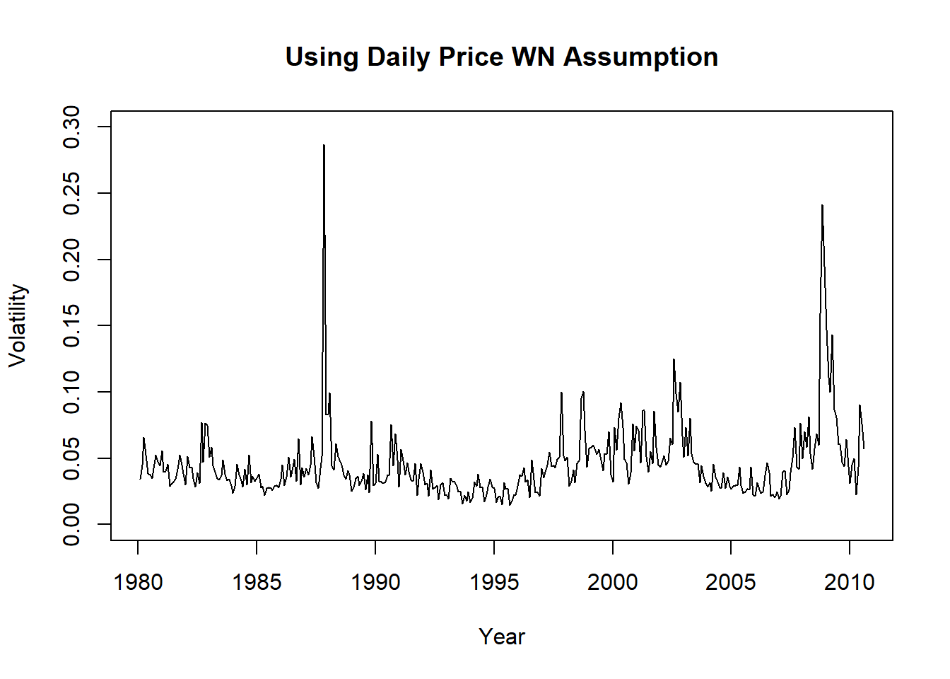
图23.1: 标普500月波动率用假定白噪声日频数据估计
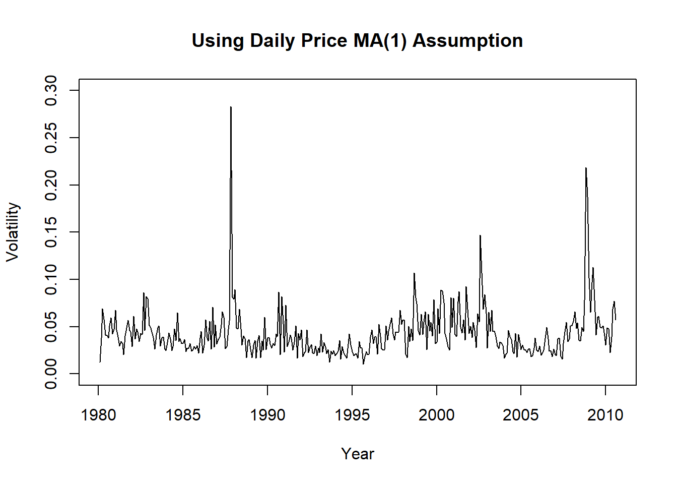
图23.2: 标普500月波动率用假定MA(1)日频数据估计
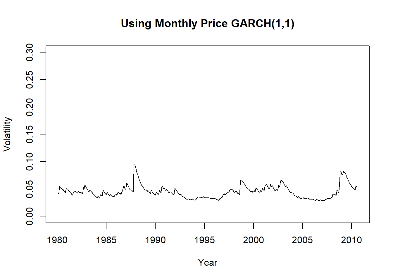
图23.3: 标普500月波动率用GARCH模型估计
可以看出日频数据估计的波动率厚尾更为严重。 将估计的三个波动率序列画在同一坐标系中:
plot(c(time(v1)), c(v1), type="l", xlab="Year",
     ylab="Volatility",
     main="Comparing 3 volatility series",
     ylim=c(0, 0.3),
     col="blue")
lines(c(time(v1)), c(v2), col="cyan")
lines(c(time(v1)), c(v3), col="black")
legend("top", lty=1, col=c("blue", "cyan", "black"),
       legend=c("日频白噪声假定", "日频MA(1)假定", "月频GARCH(1,1)估计"))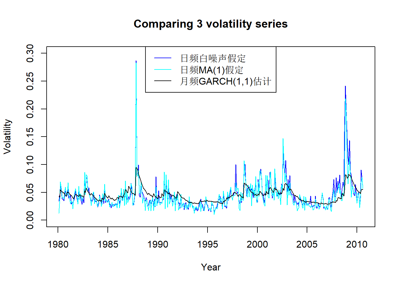
图23.4: 标普500用三种方法估计的月波动率
从图23.4看,日频数据结果仅在很高的时候比月频结果高很多, 一般情况下估计结果大小近似; 估计的走势基本一致。
比较三种方法得到的月波动率分布密度:
den1 <- density(c(v1), from=0.01, to=0.29)
den2 <- density(c(v2), from=0.01, to=0.29)
den3 <- density(c(v3), from=0.01, to=0.29)
plot(den1, xlab="Volatility", ylab="Density",
     main="Comparing 3 volatility densities",
     ylim=c(0, 40),
     col="blue")
lines(den2, col="cyan")
lines(den3, col="black")
legend("topright", lty=1, col=c("blue", "cyan", "black"),
       legend=c("日频白噪声假定", "日频MA(1)假定", "月频GARCH(1,1)估计"))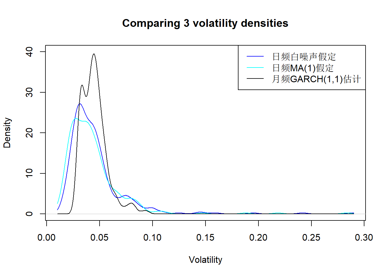
图23.5: 标普500用三种方法估计的月波动率分布密度
从图23.5可以看出日频估计的波动率更为厚尾, 月频数据估计的结果分布比较集中。 取值除了少数极端值以外, 取值范围差别不大。
23.2 使用OHLC数据
许多资产都有OHLC数据, 可以用这样的数据辅助估计波动率。
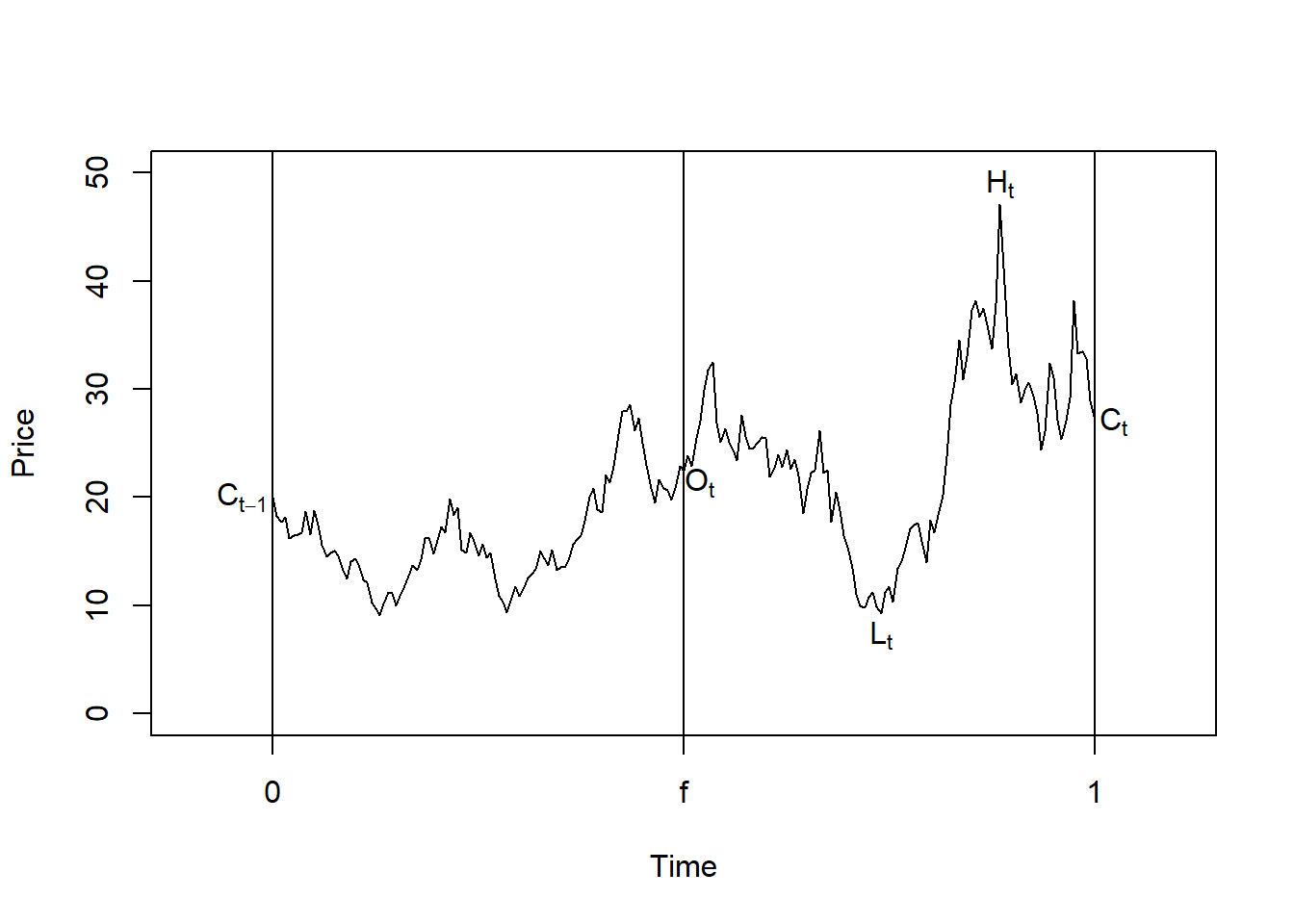
图23.6: OHLC数据形成
对于一项资产,定义如下变量:
- \(O_t\): 第\(t\)个交易日的开盘价的对数值;
- \(H_t\): 第\(t\)个交易日的最高价的对数值;
- \(L_t\): 第\(t\)个交易日的最低价的对数值;
- \(C_t\): 第\(t\)个交易日的收盘价的对数值;
- \(f\):一个自然日中闭市时间长度的比例,是一个\([0,1]\)之间的数;
- \(F_{t-1}\): 表示截止到\(t-1\)个交易日的所有公开信息, 但数学上应该是参与建模的所有可观测变量截止到\(t-1\)交易日的变量的\(\sigma\)代数。
当价格为对数价格时, 日对数收益率条件方差(波动率平方)为 \(\sigma_t^2 = E[ (C_t - C_{t-1})^2 | F_{t-1}]\)。 (假定对数收益率均值为0)。
(Garman and Klass 1980)考虑了\(\sigma_t^2\)的多种估计, 论文假定价格服从一个不带漂移的扩散过程, 可比较的估计有 \[\begin{aligned} \hat\sigma_{0t}^2 =& (C_t - C_{t-1})^2 , \\ \hat\sigma_{1t}^2 =& \frac{(O_t - C_{t-1})^2}{2f} + \frac{(C_t - O_{t})^2}{2(1-f)} , \\ \hat\sigma_{2t}^2 =& \frac{(H_t - L_t)^2}{4\ln 2} \approx 0.3607 (H_t - L_t)^2 , \\ \hat\sigma_{3t}^2 =& 0.17 \frac{(O_t - C_{t-1})^2}{f} + 0.83 \frac{(H_t - L_t)^2}{(1-f)4\ln 2} , \\ \hat\sigma_{5t}^2 =& 0.5 (H_t - L_t)^2 - (2 \ln 2 - 1) (C_t - O_t)^2 \approx 0.5 (H_t - L_t)^2 - 0.386 (C_t - O_t)^2 , \\ \hat\sigma_{6t}^2 =& 0.15 \frac{(O_t - C_{t-1})^2}{f} + 0.88 \frac{\hat\sigma_{5t}^2}{1-f} . \end{aligned}\] 其中用到\(f\)的都需要\(0<f<1\)。 论文还考虑了更复杂的\(\hat\sigma_{4t}^2\)公式, 但与\(\hat\sigma_{5t}^2\)接近。 \(\hat\sigma_{2t}^2\)估计方法是(Parkinson 1980)提出的。
定义波动率估计的效率因子为 \[\begin{aligned} \text{Eff}(\hat\sigma_{it}^2) = \frac{\text{Var}(\hat\sigma_{0t}^2)}{\text{Var}(\hat\sigma_{it}^2)} . \end{aligned}\] (Garman and Klass 1980)发现对于价格服从简单扩散模型的情形, \(i=1,2,3,5,6\)时\(\text{Eff}(\hat\sigma_{it}^2)\)分别为 2, 5.2, 6.2, 7.4和8.4, 即\(\hat\sigma_{6t}^2\)的估计效率最高。
回到对数收益率。定义
- \(o_t = O_t - C_{t-1}\)为标准化对数开盘价;
- \(u_t = H_t - O_t\)为标准化对数最高价;
- \(d_t = L_t - O_t\)为标准化对数最低价;
- \(c_t = C_t - O_t\)为标准化对数收盘价。
设有\(n\)天数据,波动率在这个期间保持恒定, (Yang and Zhang 2000)提出了如下的波动率稳健估计 \[\begin{align} \hat\sigma_{yz}^2 = \hat\sigma_o^2 + k \hat\sigma_c^2 + (1-k) \hat\sigma_{rs}^2 . \tag{23.6} \end{align}\] 其中 \[\begin{aligned} \hat\sigma_o^2 =& \frac{1}{n-1} \sum_{t=1}^n (o_t - \bar o)^2 , \\ \hat\sigma_c^2 =& \frac{1}{n-1} \sum_{t=1}^n (c_t - \bar c)^2 , \\ \hat\sigma_{rs}^2 =& \frac{1}{n} \sum_{t=1}^n \left\{ u_t (u_t - c_t) + d_t (d_t - c_t) \right\} , \\ k =& \frac{0.34}{1.34 + (n+1)/(n-1)} . \end{aligned}\] 估计\(\hat\sigma_{rs}^2\)由Rogers和Satchell(1991)提出, 选择\(k\)使得\(\hat\sigma_{yz}^2\)的标准误差最小, \(\hat\sigma_{yz}^2\)是三种估计的线性组合。
因为需要使用\(n\)天数据计算, 所以实际计算时选定一个窗宽\(n\), 每次向前滚动一天地用窗内的价格数据计算, 得到的\(\hat\sigma_{yz}^2\)作为滚动窗内最后一天的波动率平方的估计。
这些滚动计算的算法都有相位对齐问题, 一般对齐在滚动窗最后一天, 或者最后一天的下一天。 这样估计的结果一般会略有滞后, 因为最合理的对齐日期是在滚动窗的中间位置。
(Alizadeh, Brandt, and Diebold 2002)提出了用第\(t\)天的变化范围\(H_t - L_t\)估计波动率的方法。 但是实际中股票的价格仅在有交易的时刻被观测到, 所以实际的\(H_t\)和\(L_t\)可能是未被观测到的, 观测的价格变化范围可能低估了实际变化范围, 从而低估波动率。 对于交易频繁的股票, 这种偏差可以忽略; 交易不够频繁的股票则需要考虑这种偏差的影响。
23.2.1 用OHLC数据估计标普500日对数收益率的波动率
标普500指数的OHLC数据,从1980-01-03到2010-08-31, 共7737个交易日的数据。 估计日对数收益率波动率。
chartSeries(
  xts.sp5d, subset="2010-06/2010-08",
  type="bars", theme="white", TA=NULL,
  main="SP500 Daily Price",
  major.ticks="months",
  grid.ticks.on="months")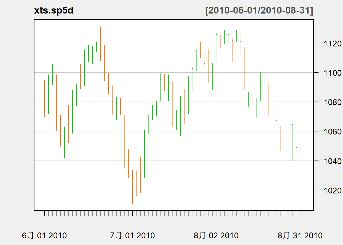
图23.7: 标普500指数序列日数据在2010年6-8月
图23.7为标普指数日数据在2010.6到8月的OHLC图形。 竖线条表示范围, 左端的短线表示开盘价, 右端的短线表示收盘价。
使用三种方法估计波动率:
- 利用Yang-Zhang方法(式(23.6)), 取滑动窗口,窗宽\(n=63\),约三个月;
- 利用Yang-Zhang方法但取\(n=32\), 与上一方法比较以查看窗宽选择对估计的影响大小;
- 为日对数收益率序列建立ARMA-GARCH模型估计波动率。
(Yang and Zhang 2000)式(23.6)估计的R函数, 利用滑动窗口计算, 计算得到的波动率的时刻与窗口最右端对齐:
## 输入x为xts类型的时间序列,bw为滑动窗口宽度
volatility.ohlc.yz <- function(x, bw=63){
  times <- index(x)
  nobs <- length(times)
  stdop <- log(Op(x)) - log(lag(Cl(x)[,1]))
  stdhi <- log(Hi(x)) - log(Op(x))
  stdlo <- log(Lo(x)) - log(Op(x))
  stdcl <- log(Cl(x)[,1]) - log(Op(x))
  k <- 0.34 / (1.34 + (bw+1)/(bw-1))

  vo <- numeric(nobs); vo[1:bw] <- NA
  vc <- vo
  vrs <- vo
  vyz <- vo

  ## 滑动计算
  for(it in (bw+1):nobs){
    ind <- (it-bw+1):it
    vo[it] <- var(stdop[ind], na.rm=TRUE)
    vc[it] <- var(stdcl[ind], na.rm=TRUE)
    vrs[it] <- 1/bw*sum(stdhi[ind]*(stdhi[ind] - stdcl[ind]) +
                          stdlo[ind]*(stdlo[ind] - stdcl[ind]))
  }
  vyz <- vo + k*vc + (1-k)*vrs

  xts(cbind(Volatility=c(sqrt(vyz))), times)
}利用式(23.6)方法, 取滑动窗口,窗口大小\(n=63\),估计波动率:
估计的波动率序列:
plot(mod4, type="l", col="red",
     ylim=c(0, 0.07),
     main="Yang-Zhang(BW=63)",
     major.ticks="years", minor.ticks=NULL,
     grid.ticks.on="years")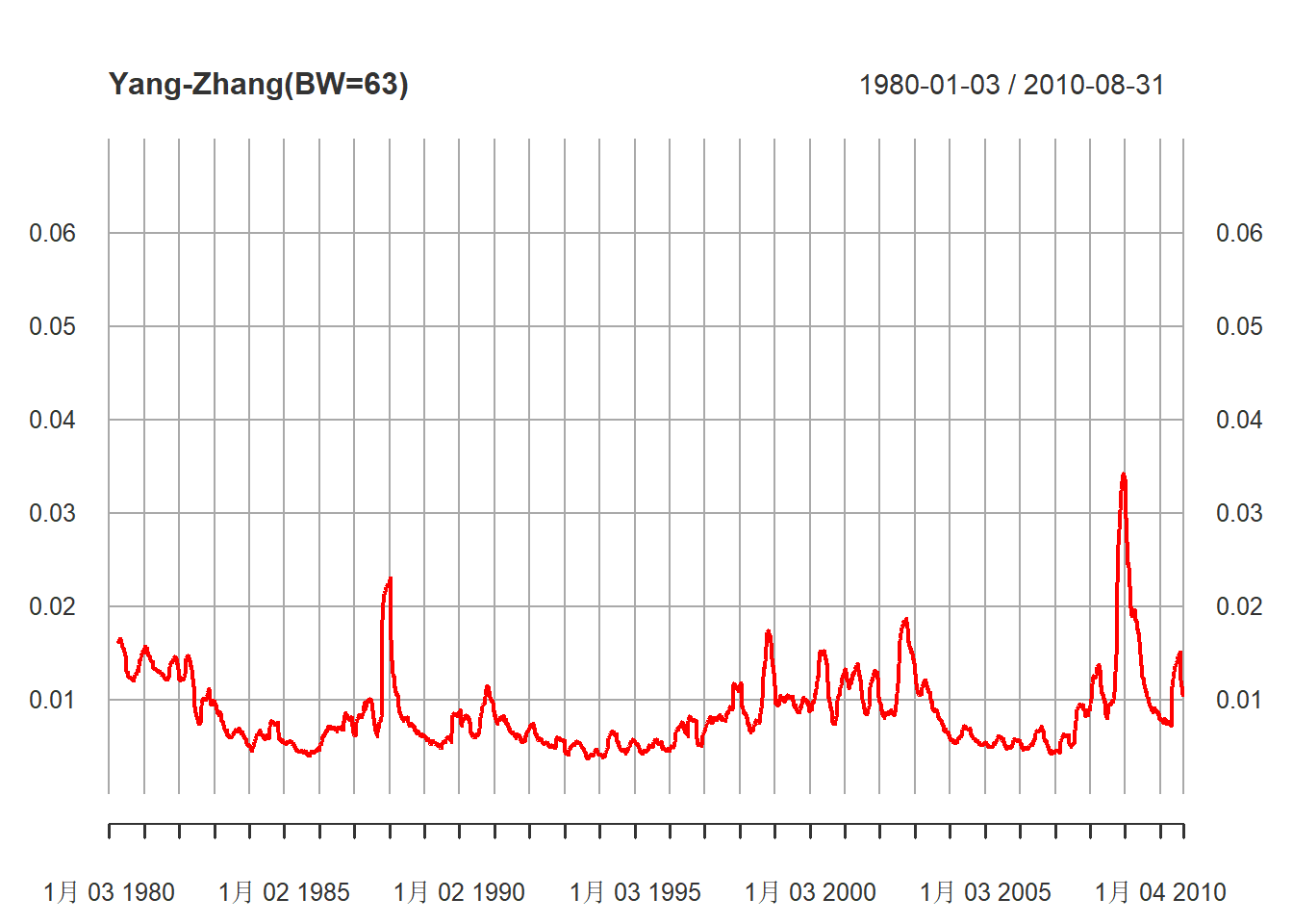
图23.8: 63天滑动计算的波动率
利用式(23.6)方法, 取滑动窗口,窗口大小\(n=32\),估计波动率:
估计的波动率序列:
plot(mod5, type="l", col="red",
     ylim=c(0, 0.07),
     main="Yang-Zhang(BW=32)",
     major.ticks="years", minor.ticks=NULL,
     grid.ticks.on="years")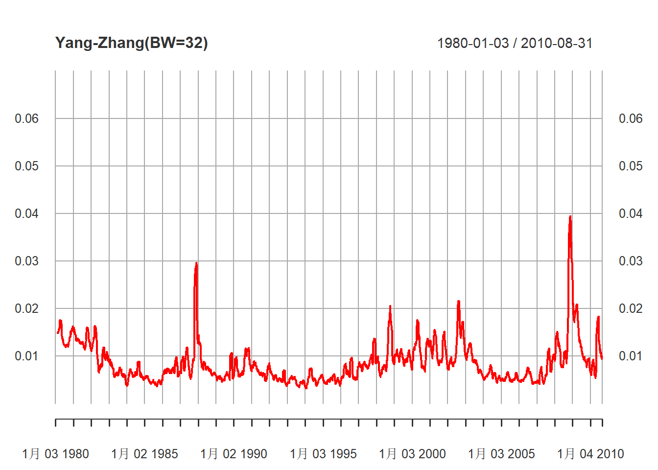
图23.9: 32天滑动计算的波动率
下面对日收盘价的对数收益率拟合一个ARMA-GARCH模型,并估计波动率。
library(fGarch, quietly = TRUE)
mod6 <- garchFit(
  ~ 1 + arma(4,0) + garch(1,1),
  data=diff(log(coredata(xts.sp5d)[,"Close",drop=TRUE])),
  trace=FALSE)
summary(mod6)
##
## Title:
## GARCH Modelling
##
## Call:
## garchFit(formula = ~1 + arma(4, 0) + garch(1, 1), data = diff(log(coredata(xts.sp5d)[,
## "Close", drop = TRUE])), trace = FALSE)
##
## Mean and Variance Equation:
## data ~ 1 + arma(4, 0) + garch(1, 1)
## <environment: 0x0000019bcc05c148>
## [data = diff(log(coredata(xts.sp5d)[, "Close", drop = TRUE]))]
##
## Conditional Distribution:
## norm
##
## Coefficient(s):
## mu ar1 ar2 ar3 ar4 omega
## 5.5450e-04 1.4467e-02 -1.1101e-02 -2.2045e-02 -3.3974e-02 1.2481e-06
## alpha1 beta1
## 7.5577e-02 9.1579e-01
##
## Std. Errors:
## based on Hessian
##
## Error Analysis:
## Estimate Std. Error t value Pr(>|t|)
## mu 5.545e-04 9.545e-05 5.810 6.26e-09 ***
## ar1 1.447e-02 1.218e-02 1.187 0.23510
## ar2 -1.110e-02 1.204e-02 -0.922 0.35655
## ar3 -2.205e-02 1.200e-02 -1.836 0.06629 .
## ar4 -3.397e-02 1.200e-02 -2.830 0.00465 **
## omega 1.248e-06 2.036e-07 6.131 8.74e-10 ***
## alpha1 7.558e-02 5.628e-03 13.428 < 2e-16 ***
## beta1 9.158e-01 6.294e-03 145.511 < 2e-16 ***
## ---
## Signif. codes: 0 '***' 0.001 '**' 0.01 '*' 0.05 '.' 0.1 ' ' 1
##
## Log Likelihood:
## 25058.57 normalized: 3.239216
##
## Description:
## Tue May 21 15:25:44 2024 by user: Lenovo
##
##
## Standardised Residuals Tests:
## Statistic p-Value
## Jarque-Bera Test R Chi^2 7046.431 0
## Shapiro-Wilk Test R W NA NA
## Ljung-Box Test R Q(10) 8.763866 0.5546507
## Ljung-Box Test R Q(15) 20.32413 0.159848
## Ljung-Box Test R Q(20) 23.147 0.2816342
## Ljung-Box Test R^2 Q(10) 3.647526 0.9618503
## Ljung-Box Test R^2 Q(15) 5.382367 0.9883641
## Ljung-Box Test R^2 Q(20) 8.517023 0.9878564
## LM Arch Test R TR^2 4.441792 0.9740826
##
## Information Criterion Statistics:
## AIC BIC SIC HQIC
## -6.476364 -6.469173 -6.476366 -6.473898估计的模型为 \[\begin{aligned} r_t =& 0.00055 + 0.0145 r_{t-1} - 0.0111 r_{t-2} - 0.0221 r_{t-3} - 0.0340 r_{t-4} + a_t, \\ a_t =& \sigma_t \varepsilon_t, \quad \varepsilon_t \sim \text{N}(0,1) \\ \sigma_t^2 =& 1.248 \times 10^{-6} + 0.0756 a_{t-1}^2 + 0.9158 \sigma_{t-1}^2 \end{aligned}\] 除了高斯分布假定外模型是充分的。 估计的波动率序列图:
plot(
  xts(volatility(mod6), index(xts.sp5d)[-1]),
  type="l", col="red",
  ylim=c(0, 0.07),
  main="ARMA-GARCH Volatility Estimate of BP500",
  major.ticks="years", minor.ticks=NULL,
  grid.ticks.on="years"
)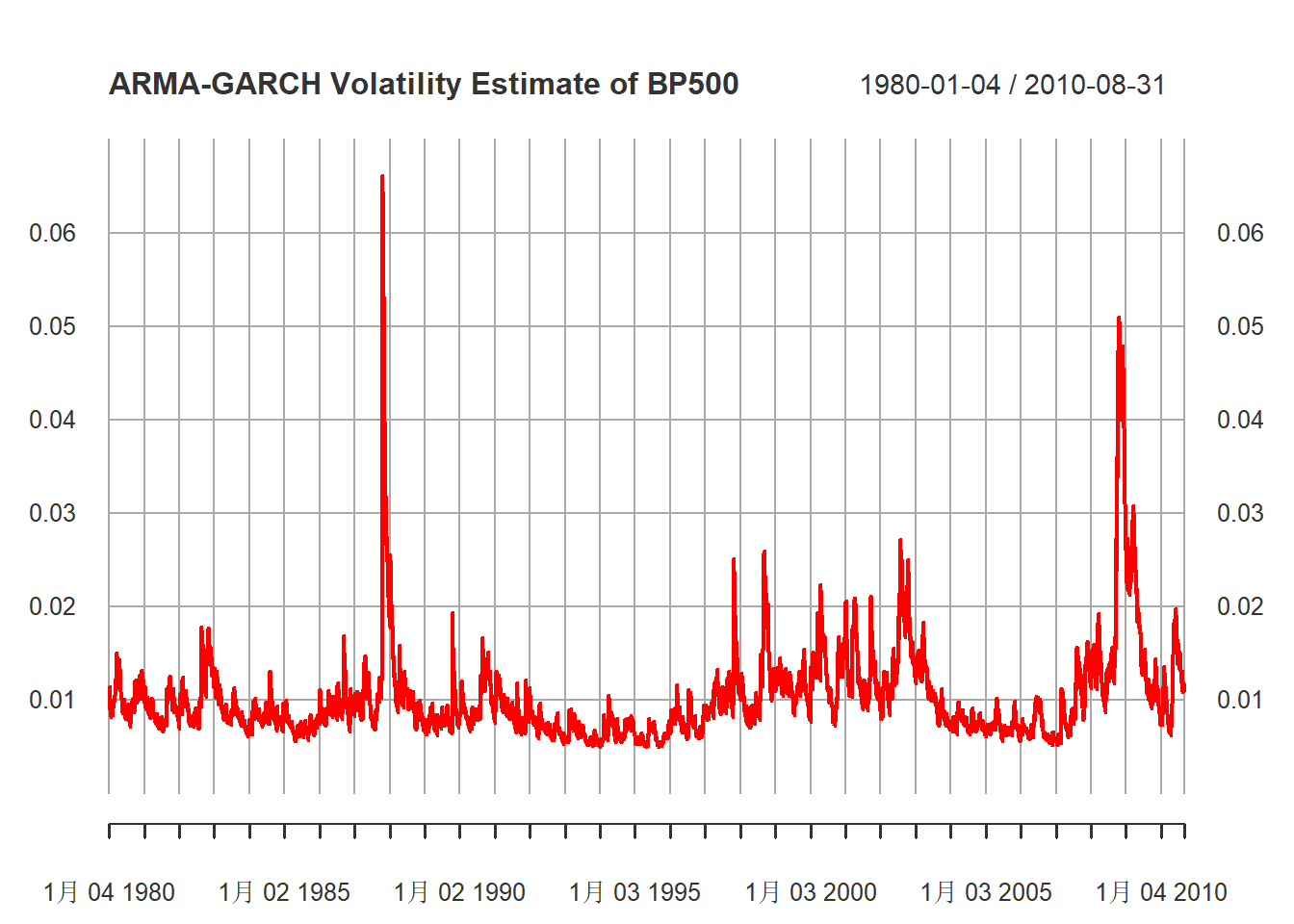
图23.10: ARMA-GARCH得到的SP500日波动率
将三种方法得到的波动率画在同一坐标系中比较:
plot(index(xts.sp5d[-1]), c(coredata(mod4))[-1],
     type="l", xlab="Year",
     ylab="Volatility",
     main="Comparing 3 volatility series",
     ylim=c(0, 0.07),
     col="blue")
lines(index(xts.sp5d[-1]), c(coredata(mod5))[-1],
      col="cyan")
lines(index(xts.sp5d[-1]), c(volatility(mod6)),
      col="black")
legend("top", lty=1, col=c("blue", "cyan", "black"),
       legend=c("Yang-Zhang BW=63", "Yang-Zhang BW=32", "ARMA-GARCH"))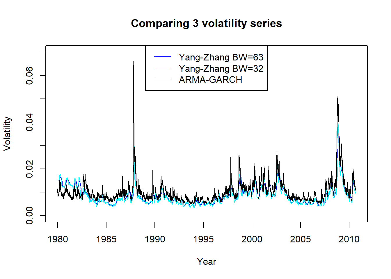
图23.11: 标普500用三种方法估计的日波动率
从图23.11看出, 三种方法估计的波动率在非极端值时比较接近, ARMA-GARCH估计的极端值更大, Yang-Zhang方法窗口宽度63和32的结果基本没有差别。
23.3 附录:用日数据估计月波动率的R函数
"vold2m" <- function(da, ma=0){
  # Compute the monthly volatility from daily prices
  # ma = 0: Assume no serial correlations in the daily returns
  # ma = 1: Assume one-lag of serial correlation in the daily returns
  # da: T-by-4 data matrix in the format [Year, Month, Day, Price]
  #
  if(!is.matrix(da)) da = as.matrix(da)
  T = nrow(da)
  pr = log(da[,4])
  rtn = c(NA, diff(pr))
  ## 不同年月个数
  nmonths <- length(unique(da[-1,1]*100 + da[-1,2]))
  vol = numeric(nmonths-1)
  cnt <- numeric(nmonths-1)

  ## x保存当前月份的收益率
  x <- numeric(31)
  id <- 0
  im <- 0
  pmon = da[2,2]
  first <- TRUE
  for (t in 2:T){
    if(da[t,2] == pmon){
      id <- id + 1
      x[id] <- rtn[t]
    } else { # new month
      if(first){
        firstmon <- c(da[t, 1:2])
        first <- FALSE
      }
      im <- im + 1
      n <- id
      v1 = n * var(x[1:n])
      v2 = 0
      if(ma==1) v2 = cov1(x[1:n])
      v1 = v1 + v2
      vol[im] <- sqrt(v1)
      cnt[im] <- n

      id <- 1
      x[1] <- rtn[t]
      pmon = da[t,2]
    }
  } # for t

  vold2m <- list(
    volatility = ts(vol, start=firstmon, frequency=12),
    ndays=cnt)
}

## 计算滞后1的中心化叉积2倍
"cov1" <- function(x){
  x[] <- x[] - mean(x)
  n <- length(x)
  2 * sum(x[1:(n-1)] * x[2:n])
}